<?xml version="1.0" encoding="utf-8"?><feed xmlns="http://www.w3.org/2005/Atom" ><generator uri="https://jekyllrb.com/" version="3.9.0">Jekyll</generator><link href="https://mlg.eng.cam.ac.uk/blog/feed.xml" rel="self" type="application/atom+xml" /><link href="https://mlg.eng.cam.ac.uk/blog/" rel="alternate" type="text/html" /><updated>2025-06-12T06:47:44+00:00</updated><id>https://mlg.eng.cam.ac.uk/blog/feed.xml</id><title type="html">MLG Blog</title><subtitle>Blog of the Machine Learning Group at the University of Cambridge</subtitle><entry><title type="html">An introduction to Flow Matching</title><link href="https://mlg.eng.cam.ac.uk/blog/2024/01/20/flow-matching.html" rel="alternate" type="text/html" title="An introduction to Flow Matching" /><published>2024-01-20T00:00:00+00:00</published><updated>2024-01-20T00:00:00+00:00</updated><id>https://mlg.eng.cam.ac.uk/blog/2024/01/20/flow-matching</id><content type="html" xml:base="https://mlg.eng.cam.ac.uk/blog/2024/01/20/flow-matching.html"><![CDATA[<style type="text/css">
/* HACK: Make the corners of the image round */
main article > img.representative-image {
  border-radius: 15px !important;
  /* HACK: gets around the `object-fit: contain` setting */
  /* Source: https://stackoverflow.com/a/70626773 */
  max-width: 100% !important;
  width: inherit;
}

/* HACK: fix overflowing mathjax */
mjx-container {
  display: inline-grid;
  overflow-x: auto;
  overflow-y: hidden;
  max-width: 100%;
}

.my-center { display: flex; }
.my-center div {
  margin: auto;
}
.my-center table {
  margin: 1em auto;
  width: inherit;
}
.my-center p { 
  width: 100%;
  text-align: center;
}
    
.my-image-container {
    padding: 5px;
}

.my-image-container img {
    border-radius: 10px;
}
    
.my-image-container p img {
    border-radius: 10px;
}

.my-small-font {
    font-size: 0.5em;
}

.my-side-by-side {
  display: inline-flex;
}

.my-danger {
  color: #a94442;
  background-color: #f2dede;
  border-color: #ebccd1;
}

.my-success {
  color: #3c763d;
  background-color: #dff0d8;
  border-color: #d6e9c6;
}

.my-warning {
  color: #8a6d3b;
  background-color: #fcf8e3;
  border-color: #faebcc;
}

.my-info {
  color: #31708f;
  background-color: #d9edf7;
  border-color: #bce8f1;
}

.my-proof {
  <!-- background-color: rgb(255, 219, 228); -->
  <!-- border-color: #bce8f1; -->
}

.my-box {
  padding: 15px;

  margin-top: 1em;
  margin-bottom: 1em;
  
  border: 1px solid transparent;
  border-radius: 4px;
}

/* Remove margins from p tags inside these boxes */
.my-box > p:first-of-type {
    margin-top: 0;
}
/ * We sometimes wrap the p tag in a div so deal with that too */
.my-box > div:first-of-type > p:first-of-type {
    margin: 0;
}
    
.my-quote {
    background-color: rgba(1, 1, 1, 0.1);
    border-radius: 5px;
    margin: 1em;
}

.my-suggestion {
    color: green;
}

.my-deletion {
    color: red;
    text-decoration: line-through;
}

main .image-container .caption {
    text-align: center;
}

/* Remove the default triangle */
summary {
  display: block;
  /* Make font a bit nicer */
  font-weight: bold;
}

/* Create a new custom triangle on the right side */
summary::after {
  margin-left: 1ch;
  display: inline-block;
  content: '▶️';
  transition: 0.2s;
}

details[open] > summary::after {
  transform: rotate(90deg);
}
</style>

\[\require{physics}
\require{color}
\newcommand{\hlorange}[1]{\colorbox{orange}{$\displaystyle#1$}}
\newcommand{\hlblue}[1]{\colorbox{blue}{$\displaystyle#1$}}
\definecolor{Highlight1}{RGB}{76,114,176}
\definecolor{Highlight2}{RGB}{85,168,104}
\definecolor{Highlight3}{RGB}{196,78,82}
\definecolor{Highlight4}{RGB}{129,114,179}
\definecolor{Highlight5}{RGB}{204,185,116}
\def\hlone#1{\color{Highlight1} #1}
\def\hltwo#1{\color{Highlight2} #1}
\def\hlthree#1{\color{Highlight3} #1}
\def\hlfour#1{\color{Highlight4} #1}
\def\hlfive#1{\color{Highlight5} #1}
\def\hlsix#1{\color{Highlight6} #1}
\def\R{\mathbb{R}}
\def\E{\mathbb{E}}
\def\P{\mathbb{P}}
\def\L{\mathcal{L}}
\def\N{\mathrm{N}}
\def\I{\mathrm{I}}
\def\Id{\mathrm{Id}}
\def\good{\color{green}{\checkmark}}
\def\bad{\color{red}{\times}}
\def\forward#1{\overset{\rightarrow}{#1}}
\def\backward#1{\overset{\leftarrow}{#1}}
\DeclareMathOperator*{\argmax}{arg\,max}
\DeclareMathOperator*{\argmin}{arg\,min}
\DeclareMathOperator*{\div}{\mathrm{div}}
\DeclareMathOperator*{\det}{\mathrm{det}}
\def\sigmamin{\sigma_{\mathrm{min}}}
\newcommand{\hlred}[1]{\colorbox{red}{$\displaystyle#1$}}
\newcommand{\hlyellow}[1]{\colorbox{yellow}{$\displaystyle#1$}}
\newcommand{\hlorange}[1]{\colorbox{orange}{$\displaystyle#1$}}
\newcommand{\hlblue}[1]{\colorbox{blue}{$\displaystyle#1$}}
\newcommand{\hlgreen}[1]{\colorbox{green}{$\displaystyle#1$}}
\nonumber\]

<h1 class="no_toc" id="table-of-contents">Table of contents</h1>

<ol id="markdown-toc">
  <li><a href="#introduction" id="markdown-toc-introduction">Introduction</a></li>
  <li><a href="#normalising-flows" id="markdown-toc-normalising-flows">Normalising Flows</a>    <ol>
      <li><a href="#learning-flow-parameters-by-maximum-likelihood" id="markdown-toc-learning-flow-parameters-by-maximum-likelihood">Learning flow parameters by maximum likelihood</a></li>
      <li><a href="#residual-flow" id="markdown-toc-residual-flow">Residual flow</a></li>
      <li><a href="#continuous-time-limit" id="markdown-toc-continuous-time-limit">Continuous time limit</a></li>
    </ol>
  </li>
  <li><a href="#flow-matching" id="markdown-toc-flow-matching">Flow matching</a>    <ol>
      <li><a href="#conditional-flows" id="markdown-toc-conditional-flows">Conditional Flows</a></li>
      <li><a href="#gaussian-probability-paths" id="markdown-toc-gaussian-probability-paths">Gaussian probability paths</a></li>
      <li><a href="#but-is-cfm-really-all-rainbows-and-unicorns" id="markdown-toc-but-is-cfm-really-all-rainbows-and-unicorns">But is CFM really all rainbows and unicorns?</a></li>
      <li><a href="#coupling" id="markdown-toc-coupling">Coupling</a></li>
    </ol>
  </li>
  <li><a href="#quick-summary" id="markdown-toc-quick-summary">Quick Summary</a></li>
  <li><a href="#citation" id="markdown-toc-citation">Citation</a></li>
  <li><a href="#acknowledgments" id="markdown-toc-acknowledgments">Acknowledgments</a></li>
  <li><a href="#references" id="markdown-toc-references">References</a></li>
</ol>

<h1 id="introduction">Introduction</h1>

<p><em>Flow matching (FM)</em> is a recent generative modelling paradigm which has rapidly been gaining popularity in the deep probabilistic ML community. Flow matching combines aspects from <em>Continuous Normalising Flows (CNFs)</em> and <em>Diffusion Models (DMs)</em>, alleviating key issues both methods have. In this blogpost we’ll cover the main ideas and unique properties of FM models starting from the basics.</p>

<h2 class="no_toc" id="generative-modelling">Generative Modelling</h2>

<p>Let’s assume we have data samples $x_1, x_2, \ldots, x_n$ from a distribution of interest $q_1(x)$, whose density is unknown. We’re interested in using these samples to learn a probabilistic model approximating $q_1$. In particular, we want efficient generation of new samples (approximately ) distributed from $q_1$. This task is referred to as <strong>generative modelling</strong>.</p>

<p>The advancement in generative modelling methods over the past decade has been nothing short of revolutionary. In 2012, Restricted Boltzmann Machines, then the leading generative model, were <a href="https://physics.bu.edu/~pankajm/ML-Notebooks/HTML/NB17_CXVI_RBM_mnist.html">just about able to generate MNIST digits</a>. Today, state-of-the-art methods are capable of generating high-quality <a href="https://openai.com/dall-e-3">images</a>, <a href="https://deepmind.google/discover/blog/transforming-the-future-of-music-creation/">audio</a> and <a href="https://arxiv.org/pdf/2305.14671.pdf">language</a>, as well as model complex <a href="https://www.nature.com/articles/s41586-023-06415-8">biological</a> and <a href="https://deepmind.google/discover/blog/nowcasting-the-next-hour-of-rain/">physical</a> systems. Unsurprisingly, these methods are now venturing into <a href="https://imagen.research.google/video/">video generation</a>.</p>

<div class="my-center">
  <div>
<div class="my-side-by-side">

      <div class="my-image-container">

        <div class="image-container">
    <img src="/blog/assets/images/flow-matching/diffusion_protein.jpg" alt="Protein generated by RFDiffusion (Watson et al., 2023)." id="figure-Figure1" style="width: 100%; max-width: 470px" />
    
        <p class="caption">
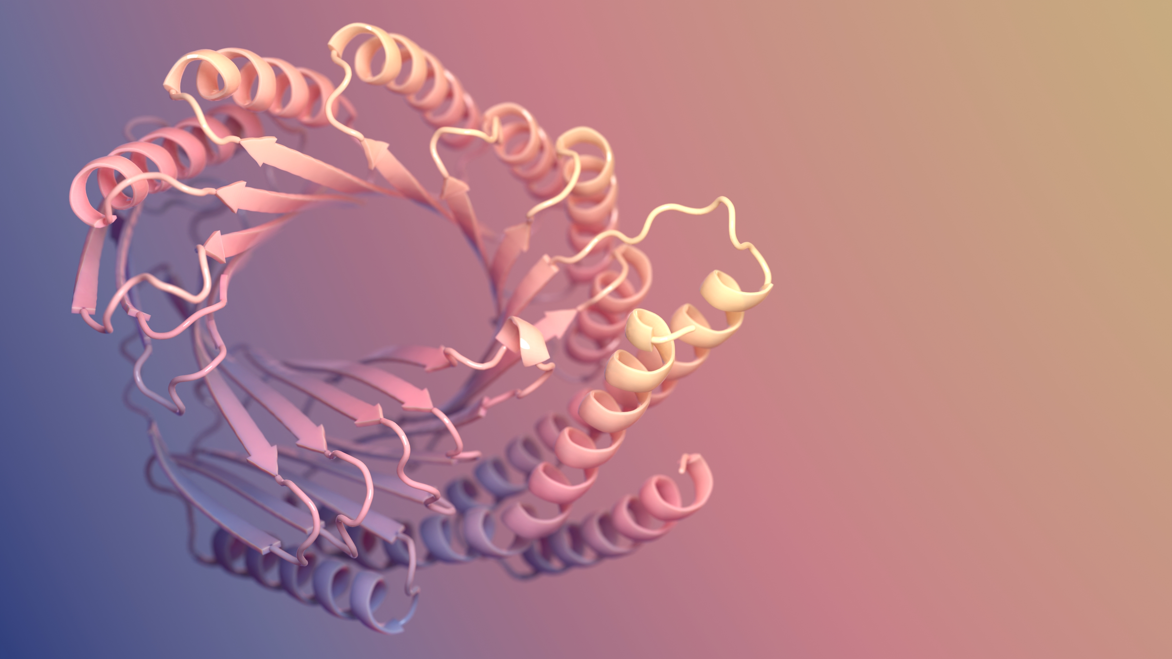
            Figure 1: Protein generated by RFDiffusion (Watson et al., 2023).
        </p>
    
</div>

      </div>
      <div class="my-image-container">

        <div class="image-container">
    <img src="/blog/assets/images/flow-matching/dalle_potatoes.jpeg" alt="Image from DALL-E 3 (Betker et al., 2023)." id="figure-Figure2" style="width: 100%; max-width: 400px" />
    
        <p class="caption">
            Figure 2: Image from DALL-E 3 (Betker et al., 2023).
        </p>
    
</div>

      </div>

    </div>
</div>
</div>

<h2 class="no_toc" id="outline">Outline</h2>

<p>Flow Matching (FM) models are in nature most closely related to (Continuous) Normalising Flows (CNFs).  Therefore, we start this blogpost by briefly recapping the core concepts behind CNFs. We then continue by discussing the difficulties of CNFs and how FM models address them.</p>

<h1 id="normalising-flows">Normalising Flows</h1>

<p>Let $\phi: \mathbb{R}^d \rightarrow \mathbb{R}^d$ be a continuously differentiable function which transforms elements of $\mathbb{R}^d$, with a continously differentiable inverse $\phi^{-1}: \mathbb{R}^d \to \mathbb{R}^d$.
Let $q_0(x)$ be a density on $\mathbb{R}^d$ and let $p_1(\cdot)$ be the density induced by the following sampling procedure</p>

\[\begin{equation*}
\begin{split}
x &amp;\sim q_0 \\
y &amp;= \phi(x),
\end{split}
\end{equation*}\]

<p>which corresponds to transforming the samples of $q_0$ by the mapping $\phi$.
Using the change-of-variable rule we can compute the density of $p_1$ as</p>

\[\begin{align}
\label{eq:changevar}
p_1(y) &amp;= q_0(\phi^{-1}(y)) \abs{\det\left[\frac{\partial \phi^{-1}}{\partial y}(y)\right]} \\
\label{eq:changevar-alt}
 &amp;= \frac{q_0(x)}{\abs{\det\left[\frac{\partial \phi}{\partial x}(x)\right]}} \quad \text{with } x = \phi^{-1}(y)
\end{align}\]

<p>where the last equality can be seen from the fact that $\phi \circ \phi^{-1} = \Id$ and a simple application of the chain rule<sup id="fnref:chainrule" role="doc-noteref"><a href="#fn:chainrule" class="footnote" rel="footnote">1</a></sup>.
The quantity $\frac{\partial \phi^{-1}}{\partial y}$ is the Jacobian of the inverse map. It is a matrix of size $d\times d$ containing $J_{ij} = \frac{d\phi^{-1}_i}{dx_j}$.
Depending on the task at hand, evaluation of likelihood or sampling, the formulation in $\eqref{eq:changevar}$ or $\eqref{eq:changevar-alt}$ is preferred (Friedman, 1987; Chen &amp; Gopinath, 2000).</p>

<details class="my-success my-box" id="example-1d-gaussian-by-linear-map">
  <summary>Example: Transformation of 1D Gaussian variables by linear map</summary>

  <div>

    <p>Suppose $\phi$ is a linear function of the form</p>

\[\phi(x) = ax+b\]

    <p>with scalar coefficients $a,b\in\mathbb{R}$, and $p$ to be Gaussian with mean $\mu$ and variance $\sigma^2$, i.e.</p>

\[p = \mathcal{N}(\mu, \sigma^2).\]

    <p>We know from linearity of Gaussians that the induced $q$ will also be Gaussian distribution but with mean $a\mu+b$ and variance $a^2 \sigma^2$, i.e.</p>

\[q = \mathcal{N}(a \mu + b, a^2 \sigma^2).\]

    <p>More interestingly, though, is to verify that we obtain the same solution by applying the change-of-variable formula.
The inverse map is given by</p>

\[\phi^{-1}(y) \mapsto \frac{y-b}{a}\]

    <p>and it’s derivative w.r.t. $y$ is thus $1/a$ assuming scalar inputs. We thus obtain</p>

\[\begin{align*}
q(y) &amp;= p\bigg(\frac{y-b}{a}\bigg) \frac{1}{a} \\
&amp;= \mathcal{N}\bigg(\frac{y-b}{a}; \mu, \sigma^2\bigg) \frac{1}{a}\\
&amp;= \frac{1}{\sqrt{2\pi\sigma^2}}\exp \bigg(-\frac{(y/a -b/a-\mu)^2}{2\sigma^2} \bigg)\frac{1}{a}\\
&amp;= \frac{1}{\sqrt{2\pi(a\sigma)^2}}\exp \bigg(-\frac{1}{a^2}\frac{(y-(a\mu+b))^2}{2\sigma^2} \bigg) \\
&amp;= \mathcal{N}\big(y; a\mu+b,a^2\sigma^2\big).
\end{align*}\]

    <p>We have thus verified that the change-of-variables formula can be used to compute the density of a Gaussian variable tranformed by a linear mapping.</p>

    <p>Often, to simplify notation, we will use the ‘push-forward’ operator $[\phi]_{\#}$ to denote the change in density of applying an invertible map $\phi$ to an input density. That is</p>

\[q(y) = ([\phi]_{\#} p)(y) = p\big(\phi^{-1}(y)\big) \det\left[\frac{\partial \phi^{-1}}{\partial y}(y)\right].\]

    <p>If we make the choice of $a = 1$ and $b = \mu$, then we get $\mathcal{N}(\mu, 1)$, as can be seen in the <a href="#figure-heatmap-colored-trajs">figure</a> below.</p>

    <!-- > [name=Emile] Same plot but without without the solid line (i.e. jumping). -->

    <div class="my-center">
      <div>
<div class="my-image-container">

          <p><!-- alt=. --></p>
          <div class="image-container">
    <img src="/blog/assets/images/flow-matching/simple-gaussian-without-trajs.png" alt="$\phi_t(x_0)$ for three samples $x_0 \sim p_0 = \mathcal{N}(0, 1)$ coloured according to $p_0(x_0)$." id="figure-heatmap-colored-trajs" style="width: 100%; max-width: 600px" />
    
        <p class="caption">
            Figure 3: $\phi_t(x_0)$ for three samples $x_0 \sim p_0 = \mathcal{N}(0, 1)$ coloured according to $p_0(x_0)$.
        </p>
    
</div>

        </div>
<div>

</div>
</div>
    </div>

  </div>

</details>

<p>Transforming a base distribution $q_0$ into another $p_1$ via a transformation $\phi$ is interesting, yet its direct application in generative modelling is limited. In generative modelling, the aim is to approximate a distribution using only the available samples. Therefore, this task requires the transformation $\phi$ to map samples from a “simple” distribution, such as $\mathcal{N}(0,I)$, to approximately the data distribution. However, a straightforward linear transformation, as in the previous example, is inadequate due to the highly non-Gaussian nature of the data distribution. This brings us to a neural network as a flexible transformation $\phi_\theta$. The key task then becomes optimising the neural net’s parameters $\theta$.</p>

<h3 id="learning-flow-parameters-by-maximum-likelihood">Learning flow parameters by maximum likelihood</h3>

<p>Let’s denote the induced parametric density by the flow $\phi_\theta$ as $p_1 \triangleq [\phi_\theta]_{\#}p_0$.</p>

<p>A natural optimisation objective for learning the parameters $\theta \in \Theta$ is to consider maximising the probability of the data under the model:</p>

\[\begin{equation*}
\textrm{argmax}_{\theta}\ \ \mathbb{E}_{x\sim \mathcal{D}} [\log p_1(x)].
\end{equation*}\]

<p>Parameterising $\phi_\theta$ as a deep neural network leads to several constraints:</p>
<ul>
  <li>How do we enforce <strong>invertibility</strong>?</li>
  <li>How do we compute its <strong>inverse</strong>?</li>
  <li>How do we compute the <strong>jacobian</strong> efficiently?</li>
</ul>

<p>Designing flows $\phi$ therefore requires trading-off expressivity (of the flow and thus of the probabilistic model) with the above mentioned considerations so that the flow can be trained efficiently.</p>

<h3 id="residual-flow">Residual flow</h3>

<p>In particular, computing the determinant of the Jacobian is in general very
expensive (as it would require $d$ automatic differentation passes in the flow) so we impose structure in $\phi$<sup id="fnref:jac_structure" role="doc-noteref"><a href="#fn:jac_structure" class="footnote" rel="footnote">2</a></sup>.</p>

<p><strong>Full-rank residual</strong> (Behrmann et al., 2019; Chen et al., 2010)</p>

<p>Expressive flows relying on a residual connection have been proposed as an interesting middle-ground between expressivity and efficient determinant estimation. They take the form:</p>

\[\begin{equation}
\label{eq:full_rank_res}
\phi_k(x) = x + \delta ~u_k(x),
\end{equation}\]

<p>where unbiased estimate of the log likelihood can be obtained<sup id="fnref:residual_flow" role="doc-noteref"><a href="#fn:residual_flow" class="footnote" rel="footnote">3</a></sup>.
As opposed to auto-regressive flows (Huang et al., 2018, Larochelle and Murray, 2011, Papamakarios et al., 2017), and low-rank residual normalising flows (Van Den Berg et al. 2018), the update in \eqref{eq:full_rank_res} has <em>full rank</em> Jacobian, typically leading to more expressive transformations.</p>

<div class="my-center">
  <div>
<div class="my-image-container">

      <div class="image-container">
    <img src="/blog/assets/images/flow-matching/jac-structure.png" alt="Jacobian structure of different normalising flows." id="figure-jac-structure.png" style="width: 100%; max-width: 600px" />
    
        <p class="caption">
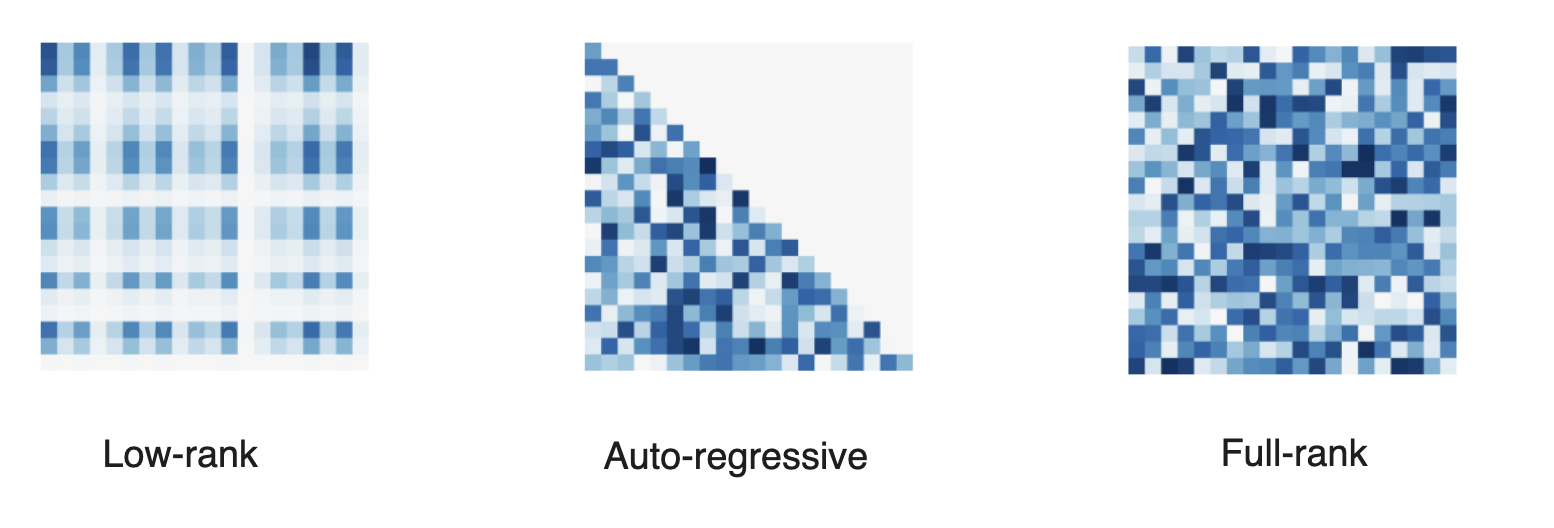
            Figure 4: Jacobian structure of different normalising flows.
        </p>
    
</div>

    </div>
</div>
</div>

<p>We can also compose such flows to get a new flow:</p>

\[\begin{equation*}
\phi = \phi_K \circ \ldots \circ \phi_2 \circ \phi_1.
\end{equation*}\]

<p>This can be a useful way to construct move expressive flows!
The model’s log-likelihood is then given by summing each flow’s contribution</p>

\[\begin{equation*}
\log q(y) = \log p(\phi^{-1}(y)) + \sum_{k=1}^K \log \det\left[\frac{\partial \phi_k^{-1}}{\partial x_{k+1}}(x_{k+1})\right]
\end{equation*}\]

<p>with $x_k = \phi_K^{-1} \circ \ldots \circ \phi^{-1}_{k} (y)$.</p>

<h3 id="continuous-time-limit">Continuous time limit</h3>
<p>As mentioned previously, residual flows are transformations of the form
$\phi(x) = x + \delta \ u(x)$
for some $\delta &gt; 0$ and Lipschitz residual connection $u$. We can re-arrange this to get</p>

\[\begin{equation*}
\frac{\phi(x) - x}{\delta} = u(x)
\end{equation*}\]

<p>which is looking awfully similar to $u$ being a derivative. In fact, letting $\delta = 1/K$ and taking the limit $K \rightarrow \infty$ under certain conditions<sup id="fnref:ODE_conditions" role="doc-noteref"><a href="#fn:ODE_conditions" class="footnote" rel="footnote">4</a></sup>, a composition of residual flows $\phi_K \circ \cdots \circ \phi_2 \circ \phi_1$ is given by an ordinary differential equation (ODE):</p>

\[\begin{equation*}
\frac{\dd x_t}{\dd t} = \lim_{\delta \rightarrow 0} \frac{x_{t+\delta} - x_t}{\delta} = \frac{\phi_t(x_t) - x_t}{\delta} = u_t(x_t)
\end{equation*}\]

<p>where the <em>flow</em> of the ODE $\phi_t: [0,1]\times\mathbb{R}^d\rightarrow\mathbb{R}^d$ is defined such that</p>

\[\begin{equation*}
\frac{d\phi_t}{dt} = u_t(\phi_t(x_0)).
\end{equation*}\]

<!--  -->
<p>That is, $\phi_t$ maps initial condition $x_0$ to the ODE solution at time $t$:</p>

\[\begin{equation*}
x_t \triangleq \phi_t(x_0) = x_0 + \int_{0}^t u_s(x_s) \dd{s} .
\end{equation*}\]

<h4 class="no_toc" id="continuous-change-in-variables">Continuous change-in-variables</h4>

<p>Of course, this only defines the map $\phi_t(x)$; for this to be a useful normalising flow, we still need to compute the log-abs-determinant of the Jacobian!</p>

<p>As it turns out, the density induced by $\phi_t$ (or equivalently $u_t$) can be computed via the following equation<sup id="fnref:FPE" role="doc-noteref"><a href="#fn:FPE" class="footnote" rel="footnote">5</a></sup></p>

\[\begin{equation*}
\frac{\partial}{\partial_t} p_t(x_t) 
= - (\nabla \cdot (u_t p_t))(x_t).
\end{equation*}\]

<!-- for some initial distribution $p_0$. -->
<p>This statement on the time-evolution of $p_t$ is generally known as the <em>Transport Equation</em>. We refer to $p_t$ as the probability path induced by $u_t$.</p>

<!-- We can also rewrite this in log-space[^log_pdf]  -->
<p>Computing the <em>total</em> derivative (as $x_t$ also depends on $t$) in log-space yields<sup id="fnref:log_pdf" role="doc-noteref"><a href="#fn:log_pdf" class="footnote" rel="footnote">6</a></sup></p>

\[\begin{equation*}
\frac{\dd}{\dd t} \log p_t(x_t) = - (\nabla \cdot u_t)(x_t)
\end{equation*}\]

<p>resulting in the log density</p>

\[\begin{equation*}
\log p_t(x) = \log p_0(x_0) - \int_0^t (\nabla \cdot u_s)(x_s) \dd{s}.
\end{equation*}\]

<p>Parameterising a vector field neural network $u_\theta: \mathbb{R}_+ \times \mathbb{R^d} \rightarrow \mathbb{R^d}$ therefore induces a parametric log-density</p>

\[\log p_\theta(x) \triangleq \log p_1(x) = \log p_0(x_0) - \int_0^1 (\nabla \cdot u_\theta)(x_t) \dd t.\]

<p>In practice, to compute $\log p_t$ one can either solve both the time evolution of $x_t$ and its log density $\log p_t$ jointly</p>

\[\begin{equation*}
\frac{\dd}{\dd t} \Biggl( \begin{aligned} x_t \ \quad \\ \log p_t(x_t) \end{aligned} \Biggr) = \Biggl( \begin{aligned} u_\theta(t, x_t) \quad \\ - \div u_\theta(t, x_t) \end{aligned} \Biggr),
\end{equation*}\]

<p>or solve only for $x_t$ and then use quadrature methods to estimate $\log p_t(x_t)$.</p>

<p>Feeding this (joint) vector field to an adaptive step-size ODE solver allows us to control both the error in the sample $x_t$ and the error in the $\log p_t(x)$.</p>

<p>One may legitimately wonder why should we bother with such <em>time-continuous</em> flows versus <em>discrete</em> residual flows. There are a couple of benefits:</p>
<ol>
  <li>CNFs can be seen as an automatic way of choosing the number of residual flows $K$ to use, which would otherwise be a hyperparameter we would have to tune. In the time-continuous setting, we can choose an error threshold $\epsilon$ and the adapative solver would give us a the discretisation step size $\delta$, effectively yielding $K = 1/\delta$ steps. Using an explicit first order solver, each step is of the form $x \leftarrow x + \delta \ u_\theta(t_k, x)$, akin to a residual flow, where the residual connection parameters $\theta$ are <em>shared</em> for each discretisation step, since $u_\theta$ is amortised over $t$, instead of having a different $\theta_k$ for each layer.</li>
  <li>In residual flows, during training we need to ensure that $u_\theta$ is $1 / \delta$ Lipschitz; otherwise the resulting flow will not be invertible and thus not a valid normalising flow. With CNFs, we still require the vector field $u_\theta(t, x)$ to be Lipschitz in $x$, <em>but</em> we don’t have to worry about exactly what this Lipschitz constant is, which is obviously much easier to satisfy and enforce in the neural architecture.
<!-- , as an adaptive ODE solver will automatically choose a suitable step size $\delta$ for us. --></li>
</ol>

<!-- > [name=Tor] Regarding "residual connection parameters $\theta$ are *shared* for each discretisation step", there is nothing stopping us from having the paameters depend on $t$ in a way that recovers the behavior we would see in a discrete case, no? -->

<p>Now that you know why CNFs are cool, let’s have a look at what such a flow would be for a simple example.</p>

<details class="my-success my-box" id="example-gaussian-to-gaussian">
  <summary>
Example: Gaussian to a Gaussian (1D)
</summary>

  <div>
    <p>Let’s come back to our earlier example of mapping a 1D Gaussian to another one with different mean.
In contrast to previously where we derived a ‘one-shot’ (i.e. <em>discrete</em>) flow bridging between the two Gaussians, we now aim to derive a time-<em>continuous flow</em> $\phi_t$ which would correspond to the time integrating a vector field $u_t$.</p>

    <!-- Before digging into how exactly we achieve this, it is useful to consider an example of the above correspondance $\phi(t, x) \longleftrightarrow u(t, x)$ can be determined in closed-form. Let's consider the simple scenario we saw earlier where we want to bridge -->
    <p>We have the following two distributions</p>

\[\begin{equation*}
p_0 = \mathcal{N}(0, 1) \quad \text{and} \quad p_1 = \mathcal{N}(\mu, 1).
\end{equation*}\]

    <!-- i.e two simple Gaussians but with different means. -->

    <!-- It's not difficult to see how we can achieve this with a simple linear transformation, e.g. -->
    <p>It’s not difficult to see that we can continuously bridge between these with a simple linear transformation</p>

\[\begin{equation*}
\phi(t, x_0) = x_0 + \mu t
\end{equation*}\]

    <p>which is visualized in the figure below.</p>

    <div class="my-center">
      <div>
<div class="my-image-container">

          <div class="image-container">
    <img src="/blog/assets/images/flow-matching/heatmap-colored-trajs.png" alt="$\phi_t(x_0)$ for a few samples $x_0 \sim p_0 = \mathcal{N}(0, 1)$ coloured according to $p_0(x_0)$." id="figure-heatmap-colored-trajs.png" style="width: 100%; max-width: 600px" />
    
        <p class="caption">
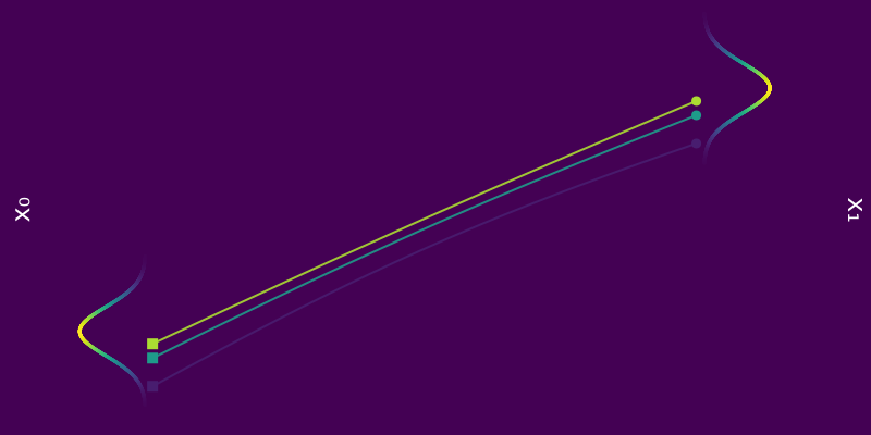
            Figure 5: $\phi_t(x_0)$ for a few samples $x_0 \sim p_0 = \mathcal{N}(0, 1)$ coloured according to $p_0(x_0)$.
        </p>
    
</div>

        </div>
<div>
    
    
</div>
</div>
    </div>

    <p>By linearity, we know that every marginal $p_t$ is a Gaussian, and so</p>

\[\begin{equation*}
\mathbb{E}_{p_0}[\phi_t(x_0)] = \mu t
\end{equation*}\]

    <p>which, in particular, implies that $\mathbb{E}_{p_0}[\phi_1(x_0)] = \mu = \mathbb{E}_{p_1}[x_1]$. Similarly, we have</p>

\[\begin{equation*}
\mathrm{Var}_{p_0}[\phi_t(x_0)] = 1 \quad \implies \quad \mathrm{Var}_{p_0}[\phi_1(x_0)] = 1 = \mathrm{Var}_{p_1}[x_1]
\end{equation*}\]

    <p>Hence we have a probability path $p_t = \mathcal{N}(\mu t, 1)$ bridging $p_0$ and $p_1$.</p>

    <div class="my-center">
      <div>
<div class="my-image-container">

          <div class="image-container">
    <img src="/blog/assets/images/flow-matching/heatmap-colored.png" alt="Probability path $p_t = \mathcal{N}(\mu t, 1)$ from $p_0 = \mathcal{N}(0, 1)$ to $p_1 = \mathcal{N}(\mu, 1)$." id="figure-heatmap-colored.png" style="width: 100%; max-width: 600px" />
    
        <p class="caption">
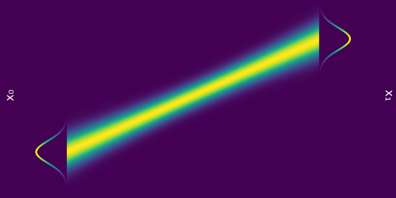
            Figure 6: Probability path $p_t = \mathcal{N}(\mu t, 1)$ from $p_0 = \mathcal{N}(0, 1)$ to $p_1 = \mathcal{N}(\mu, 1)$.
        </p>
    
</div>

        </div>

<div>
    

</div>
</div>
    </div>

    <!-- > [name=emilem] Would be nice to ideally shorten what follows. -->

    <p>Now let’s determine what the vector field $u_t(x)$ would be in this case. As mentioned earlier, $u(t, x)$ should satisfy the following</p>

\[\begin{equation*}
\dv{\phi_t}{t}(x_0) = u_t \big( \phi_t(x_0) \big).
\end{equation*}\]

    <p>Since we have already specified $\phi$, we can plug it in on the left hand side to get</p>

\[\begin{equation*}
\dv{\phi_t}{t}(x_0) = \dv{t} \big( x_0 + \mu t \big) = \mu
\end{equation*}\]

    <p>which gives us</p>

\[\begin{equation*}
\mu = u_t \big( x_0 + \mu t \big).
\end{equation*}\]

    <p>The above needs to hold for <em>all</em> $t \in [0, 1]$, and so it’s not too difficult to see that one such solution is the constant vector field</p>

\[\begin{equation*}
u_t(x) = \mu.
\end{equation*}\]

    <p>We could of course have gone the other way, i.e. define the $u_t$ such that $p_0 \overset{u_t}{\longleftrightarrow} p_1$ and derive the corresponding $\phi_t$ by solving the ODE.</p>

  </div>

</details>

<h4 class="no_toc" id="training-cnfs">Training CNFs</h4>

<p>Similarly to any flows, CNFs can be trained by maximum log-likelihood</p>

\[\mathcal{L}(\theta) = \mathbb{E}_{x\sim q_1} [\log p_1(x)],\]

<p>where the expectation is taken over the data distribution and $p_1$ is the parameteric distribution.
This involves integrating the time-evolution of samples $x_t$ and log-likelihood $\log p_t$, both terms being a function of the parametric vector field $u_{\theta}(t, x)$. This requires</p>

<ul>
  <li>⚠️ Expensive numerical ODE simulations at training time!</li>
  <li>⚠️ Estimators for the divergence to scale nicely with high dimension. <sup id="fnref:hutchinson" role="doc-noteref"><a href="#fn:hutchinson" class="footnote" rel="footnote">7</a></sup></li>
</ul>

<p>CNFs are very expressive as they parametrise a large class of flows, and therefore of probability distributions. Yet training can be <em>extremely</em> slow due to the ODE integration at each iteration. One may wonder whether a ‘simulation-free’, i.e. <em>not</em> requiring any integration, training procedure exists for training these CNFs.</p>

<!-- > [name=Tor] Should add a citation for the "large class of flows" claim. -->

<h1 id="flow-matching">Flow matching</h1>

<p>And that is exactly where Flow Matching (FM) comes in!</p>

<!--- 
Here comes flow matching achieving exactly this, 
-->
<p>Flow matching is a simulation-free way to train CNF models where we directly formulate a regression objective w.r.t. the parametric vector field $u_\theta$ of the form
<!-- \label{eq:fm-objective} --></p>

\[\begin{equation*}
\mathcal{L}(\theta)_{} = \mathbb{E}_{t \sim \mathcal{U}[0, 1]} \mathbb{E}_{x \sim p_t}\left[\|
u_\theta(t, x) - u(t, x) \|^2 \right].
\end{equation*}\]

<p>In the equation above, $u(t, x)$ would be a vector field inducing a <em>probability path</em> (or bridge) $p_t$ interpolating the reference $p_0$ to $p_1$, i.e.</p>

\[\begin{equation*}
\log p_1(x) = \log p_0 - \int_0^1 (\nabla \cdot u_t)(x_t) \dd{t}.
\end{equation*}\]

<!-- $$
\begin{equation*}
\pdv{p_t(x)}{t} = - \nabla \cdot \big( u_t(x) p_t(x) \big),
\end{equation*}
$$ -->

<p>In words: we’re just performing regression on $u_t(x)$ for all $t \in [0, 1]$.</p>

<p>Of course, this requires knowledge of a <em>valid</em> $u(t, x)$, and if we already have access to $u_t$, there’s no point in learning an approximation $u_{\theta}(t, x)$ in the first place! But as we will see in the next section, we can leverage this formulation to construct a useful target for $u_{\theta}(t, x)$ witout having to compute explicitly $u(t, x)$.</p>

<p>This is where <em>Conditional</em> Flow Matching (CFM) comes to the rescue.</p>

<details class="my-info my-box" open="true">
  <summary>
Non-uniqueness of vector field
</summary>

  <div>

    <p>We say <em>a valid</em> $u_t$ because there is no <em>unique</em> vector field $u_t$; there are indeed many valid choices for $u_t$ inducing maps $p_0 \overset{\phi}{\longleftrightarrow} p_1$ as illustrated in the <a href="#figure-forward_samples-one-color-1">figure</a> below. As we will see in what follows, in practice we have to pick a particular target $u_t$, which has practical implications.
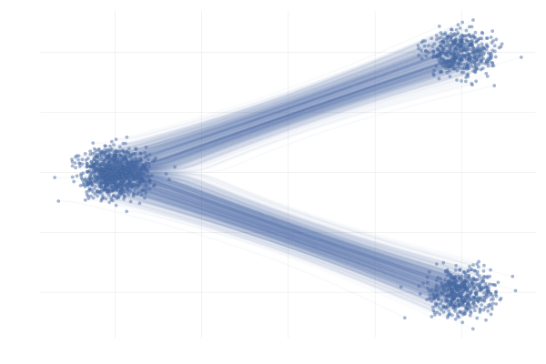
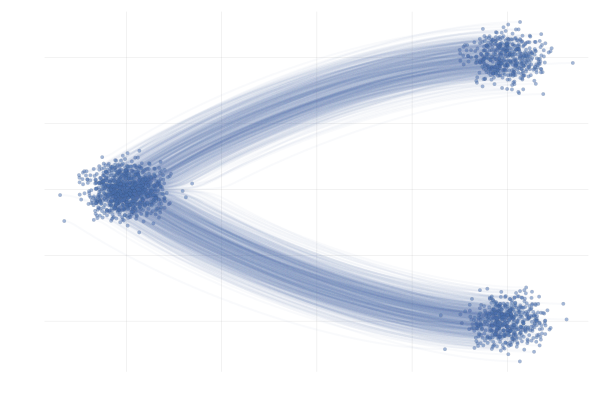
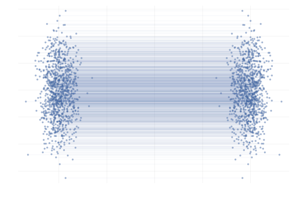
</p>

  </div>

  <div class="my-center">
    <div>
<div class="my-side-by-side">
        <div class="my-image-container">

          <div class="image-container">
    <img src="/blog/assets/images/flow-matching/forward_samples-one-color-1.png" alt="" id="figure-forward_samples-one-color-1" style="width: 100%; max-width: 400px" />
    
</div>

          <!-- $$
\phi_t(x_0, x_1) = (1 - t) x_0 + t x_1
$$ -->

        </div>
        <div class="my-image-container">

          <div class="image-container">
    <img src="/blog/assets/images/flow-matching/forward_samples-one-color-2.png" alt="" id="figure-forward_samples-one-color-2.png" style="width: 100%; max-width: 400px" />
    
</div>

          <!-- $$
\phi_t(x_0, x_1) = \cos(\pi t / 2) x_0 + \sin (\pi t / 2) x_1
$$ -->

        </div>
      </div>

<div>

<!-- Figure: Different paths with the same endpoints -->
<!-- $p_0 = \mathcal{N}([- \mu, 0], I)$ and $p_1 = \frac{1}{2} \mathcal{N}([\mu, \mu], I) + \frac{1}{2} \mathcal{N}([\mu, - \mu], I)$ -->
</div>
</div>
  </div>

  <div class="my-center">
    <div>
<div class="my-side-by-side">
        <div class="my-image-container">

          <div class="image-container">
    <img src="/blog/assets/images/flow-matching/forward_samples-one-color-3.png" alt="" id="figure-forward_samples_ot-one-color.png" style="width: 100%; max-width: 400px" />
    
</div>

        </div>
        <div class="my-image-container">

          <div class="image-container">
    <img src="/blog/assets/images/flow-matching/forward_samples_ot-one-color.png" alt="" id="figure-forward_samples-one-color-3.png" style="width: 100%; max-width: 400px" />
    
</div>

        </div>
      </div>
<div>

<p class="caption">

Figure 7: <em>Different paths with the same endpoints marginals<sup id="fnref:interpolation" role="doc-noteref"><a href="#fn:interpolation" class="footnote" rel="footnote">8</a></sup>.</em>

</p>
<!-- $p_0 = p_1 = \mathcal{N}(0, I)$.* -->

</div>
</div>
  </div>

</details>

<!-- > [name=Tor Erlend Fjelde] TODO: add footnote on details. -->

<h3 id="conditional-flows">Conditional Flows</h3>

<p>First, let’s remind ourselves that the transport equation relates a vector field $u_t$ to (the time evolution of) a probability path $p_t$</p>

\[\begin{equation*}
\pdv{p_t(x)}{t} = - \nabla \cdot \big( u_t(x) p_t(x) \big),
\end{equation*}\]

<p>thus constructing $p_t$ or $u_t$ is <em>equivalent</em>.
One key idea (Lipman et al., 2023 and Albergo &amp; Vanden-Eijnden, 2022) is to express the probability path as a marginal over a joint involving a latent variable $z$: 
$p_t(x_t) = \int p(z) ~p_{t\mid z}(x_t\mid z) \textrm{d}z$.
The $p_{t\mid z}(x_t\mid z)$ term being a <strong>conditional probability path</strong>, satisfying some boundary conditions at $t=0$ and $t=1$ so that $p_t$ be a valid path interpolating between $q_0$ and $q_1$.
In addition, as opposed to the marginal $p_t$ , the conditional $p_{t\mid1}$ could be available in closed-form.</p>

<p>In particular, as we have access to data samples $x_1 \sim q_1$, it sounds pretty reasonable to condition on $z=x_1$, leading to the following marginal probabilithy path</p>

\[\begin{equation*}
p_t(x_t) = \int q_1(x_1) ~p_{t\mid 1}(x_t\mid x_1) \dd{x_1}.
\end{equation*}\]

<!-- would interpolate between $p_{t=0} = q_0$ and $p_{t=1}=\delta_{x_1}$.  -->
<p>In this setting, the conditional probability path $p_{t\mid 1}$ needs to satisfy the boundary conditions</p>

\[\begin{equation*}
p_0(x \mid x_1) = p_0 \quad \text{and} \quad p_1(x \mid x_1) = \mathcal{N}(x; x_1, \sigmamin^2 I) \xrightarrow[\sigmamin \rightarrow 0]{} \delta_{x_1}(x)
\end{equation*}\]

<p>with $\sigmamin &gt; 0$ small, and for whatever reference $p_0$ we choose, typically something “simple” like $p_0(x) = \mathcal{N}(x; 0, I)$, as illustrated in the <a href="#figure-heatmap_with_cond_traj-v3">figure</a> below.</p>

<div class="my-center">
  <div class="my-image-container">

    <div class="image-container">
    <img src="/blog/assets/images/flow-matching/heatmap_with_cond_traj-v3.png" alt="Two conditional flows $\phi_t(x \mid x_1)$ for two univariate Gaussians." id="figure-heatmap_with_cond_traj-v3" style="width: 100%; max-width: 600px" />
    
        <p class="caption">
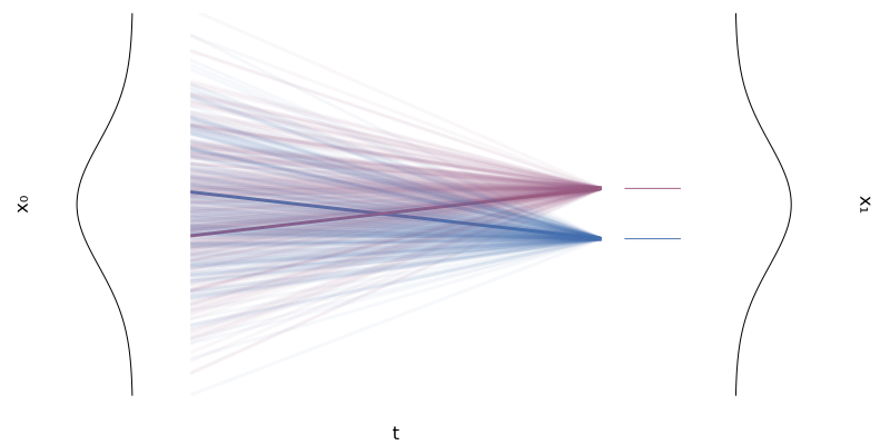
            Figure 8: Two conditional flows $\phi_t(x \mid x_1)$ for two univariate Gaussians.
        </p>
    
</div>

  </div>
</div>

<p>The conditional probability path also satisfies the transport equation with the <strong>conditional vector field</strong> $u_t(x \mid x_1)$:</p>

\[\begin{equation}
\label{eq:continuity-cond}
\pdv{p_t(x \mid x_1)}{t} = - \nabla \cdot \big( u_t(x \mid x_1) p_t(x \mid x_1) \big).
\end{equation}\]

<!-- Lipman et al. (2023) introduced the notion of **Conditional Flow Matching (CFM)** by noticing that the *conditional* vector field $u_t(x \mid x_1)$, which satisfies the transport equation for the conditional density $p_t(x \mid x_1)$
\label{eq:continuity-cond-2}
$$
\begin{equation*}
\pdv{p_t(x \mid x_1)}{t} = - \nabla \cdot \big( u_t(x \mid x_1) p_t(x \mid x_1) \big),
\end{equation*}
$$
 -->
<p>Lipman et al. (2023) introduced the notion of <strong>Conditional Flow Matching (CFM)</strong> by noticing that this <em>conditional</em> vector field $u_t(x \mid x_1)$
can express the <em>marginal</em> vector $u_t(x)$ of interest via the conditional probability path $p_{t\mid 1}(x_t\mid x_1)$ as</p>

\[\begin{equation}
\label{eq:cf-from-cond-vf}
\begin{split}
  u_t(x) &amp;= \mathbb{E}_{x_1 \sim p_{1 \mid t}} \left[ u_t(x \mid x_1) \right] \\
  &amp;= \int u_t(x \mid x_1) \frac{p_t(x \mid x_1) q_1(x_1)}{p_t(x)} \dd{x}_1.
\end{split}
\end{equation}\]

<!-- That is, we have an unbiased estimator the marginal vector field $u_t$ that we want to learn by sampling $x_1$ from $p_{1 \mid t}(x_1 \mid x)$ and evaluating $u_t(x \mid x_1)$. -->

<p>To see why this $u_t$ the same the vector field as the one defined earlier, i.e. the one generating the (marginal) probability path $p_t$, we need to show that the expression above for the marginal vector field $u_t(x)$ satisfies the transport equation</p>

\[\begin{equation*}
\pdv{\hlthree{p_t(x)}}{t} = - \nabla \cdot \big( \hltwo{u_t(x)} \hlthree{p_t(x)} \big).
\end{equation*}\]

<p>Writing out the left-hand side, we have</p>

\[\begin{equation*}
\begin{split}
  \pdv{\hlthree{p_t(x)}}{t} &amp;= \pdv{t} \int p_t(x \mid x_1) q(x_1) \dd{x_1} \\
  &amp;= \int \hlone{\pdv{t} \big( p_t(x \mid x_1) \big)} q(x_1) \dd{x_1} \\
  &amp;= - \int \hlone{\nabla \cdot \big( u_t(x \mid x_1) p_t(x \mid x_1) \big)} q(x_1) \dd{x_1} \\
  &amp;= - \int \hlfour{\nabla} \cdot \big( u_t(x \mid x_1) p_t(x \mid x_1) q(x_1) \big) \dd{x_1} \\
  &amp;= - \hlfour{\nabla} \cdot \int u_t(x \mid x_1) p_t(x \mid x_1) q(x_1) \dd{x_1} \\
  &amp;= - \nabla \cdot \bigg( \int u_t(x \mid x_1) \frac{p_t(x \mid x_1) q(x_1)}{\hlthree{p_t(x)}} {\hlthree{p_t(x)}} \dd{x_1} \bigg) \\
  &amp;= - \nabla \cdot \bigg( {\hltwo{\int u_t(x \mid x_1) \frac{p_t(x \mid x_1) q(x_1)}{p_t(x)} \dd{x_1}}} \ {\hlthree{p_t(x)}} \bigg) \\
  &amp;= - \nabla \cdot \big( \hltwo{u_t(x)} {\hlthree{p_t(x)}} \big)
\end{split}
\end{equation*}\]

<p>where in the $\hlone{\text{first highlighted step}}$ we used \eqref{eq:continuity-cond} and in the $\hltwo{\text{last highlighted step}}$ we used the expression of $u_t(x)$ in \eqref{eq:cf-from-cond-vf}.</p>

<p>The relation between $\phi_t(x_0)$, $\phi_t(x_0 \mid x_1)$ and their induced densities are illustrated in the <a href="#figure-flow-matching-diagram">Figure 9</a> below. And since $\phi_t(x_0)$ and $\phi_t(x_0 \mid x_1)$ are solutions corresponding to the vector fields $u_t(x)$ and $u_t(x \mid x_1)$ with $x(0) = x_0$, <a href="#figure-flow-matching-diagram">Figure 9</a> is equivalent to <a href="#figure-flow-matching-diagram-2">Figure 10</a>, but note the difference in the expectation taken to go from $u_t(x_0 \mid x_1) \longrightarrow u_t(x_0)$ compared to $\phi_t(x_0 \mid x_1) \longrightarrow \phi_t(x_0)$.</p>

<div class="my-center">
  <div>
<div class="my-image-container">

      <div class="image-container">
    <img src="/blog/assets/images/flow-matching/flow-matching-diagram.png" alt="Diagram illustrating the relation between the paths $\phi_t(x_0)$, $\phi_t(x_0 \mid x_1)$, and their induced marginal and conditional densities." id="figure-flow-matching-diagram" style="width: 100%; max-width: 500px" />
    
        <p class="caption">
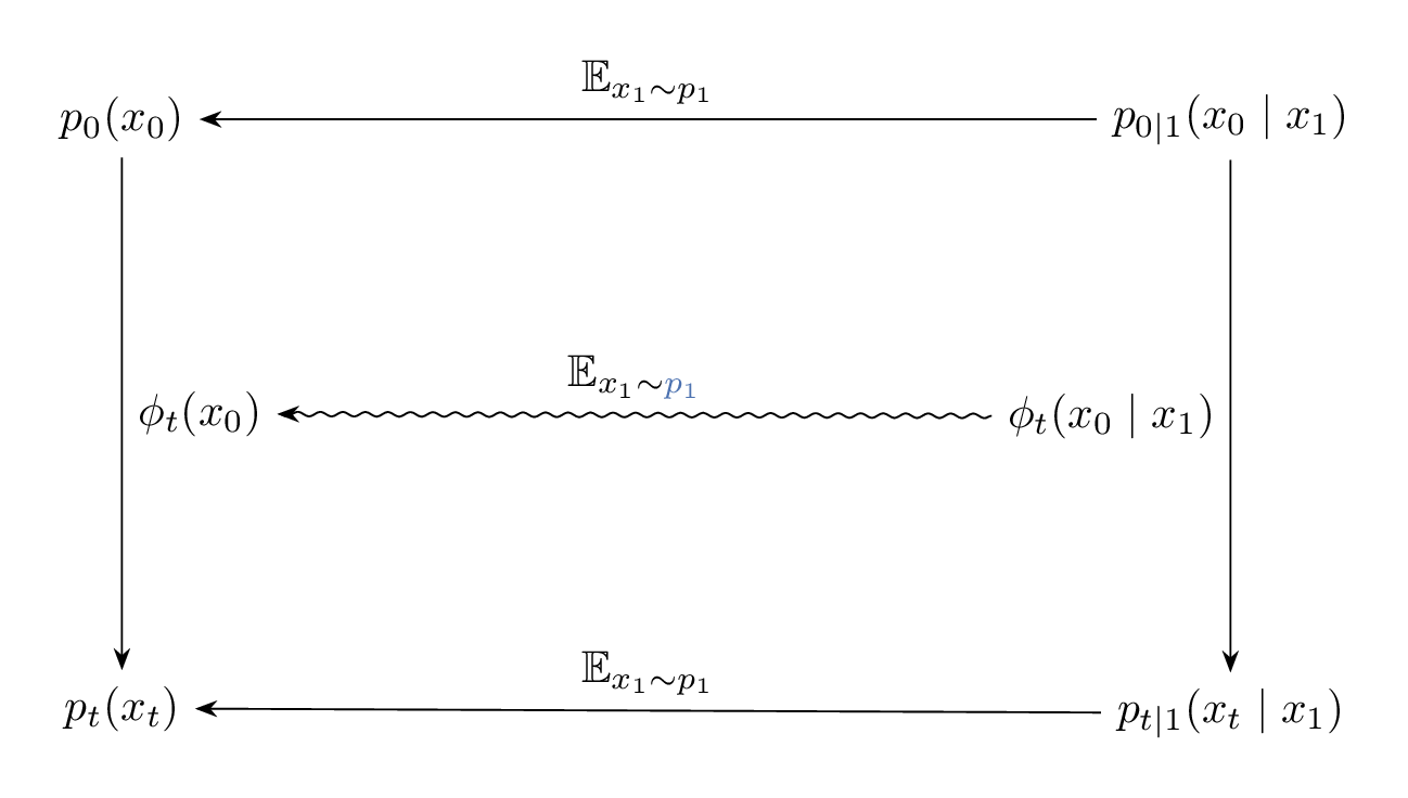
            Figure 9: Diagram illustrating the relation between the paths $\phi_t(x_0)$, $\phi_t(x_0 \mid x_1)$, and their induced marginal and conditional densities.
        </p>
    
</div>

    </div>
</div>
</div>

<div class="my-center">
  <div>
<div class="my-image-container">

      <div class="image-container">
    <img src="/blog/assets/images/flow-matching/flow-matching-diagram-2.png" alt="Diagram illustrating the relation between the vector fields $u_t(x_0)$, $u_t(x_0 \mid x_1)$, and their induced marginal and conditional densities." id="figure-flow-matching-diagram-2" style="width: 100%; max-width: 700px" />
    
        <p class="caption">
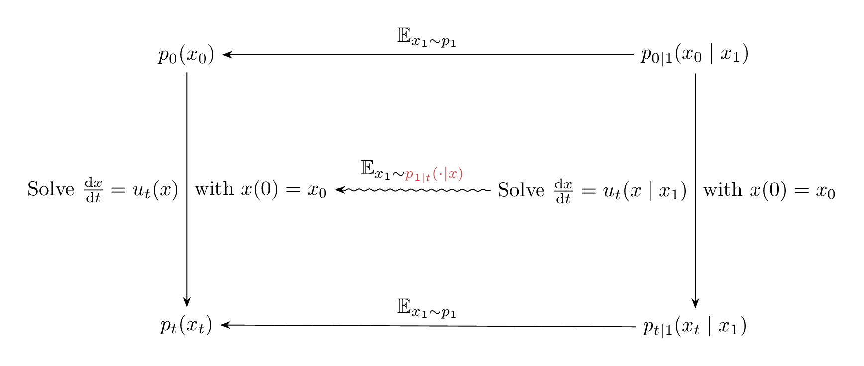
            Figure 10: Diagram illustrating the relation between the vector fields $u_t(x_0)$, $u_t(x_0 \mid x_1)$, and their induced marginal and conditional densities.
        </p>
    
</div>

    </div>
</div>
</div>

<details class="my-info my-box" open="true">
  <summary>
Gaussian to Gaussian (2D) using a conditional flow
</summary>

  <div>

    <p>Let’s try to gain some intuition behind \eqref{eq:cf-from-cond-vf} and the relation between $u_t(x)$ and $u_t(x \mid x_1)$.
We do so by looking at the following scenario</p>

    <!-- Suppose we have some data samples $\big( x_1^{(i)} \big)_{i = 1}^n$ from our target $p_1$.
For any point $x$ in our domain, we can produce an unbiased estimate of $u_t(x)$ by
$$
\begin{split}
u_t \big( x \big) &= \mathbb{E}_{x_1 \sim p_1} \left[ u_t \big( x \mid x_1 \big) \frac{p_t(x \mid x_1)}{p_t(x)} \right] \\
&\approx \frac{1}{n} \sum_{i = 1}^n u_t \big( x \mid x_1^{(i)} \big) \frac{p_t(x \mid x_1^{(i)})}{p_t(x)}.
\end{split}
$$
assuming we could compute the weights $\frac{p_t(x \mid x_1^{(i)})}{p_t(x)}$, we could use importance sampling (IS) to estimate $u_t(x)$ from $u_t(x \mid x_1)$ and samples from $p_1$. In effect, the IS weight $\frac{p_t(x \mid x_1^{(i)})}{p_t(x)}$ tells us how important the sample $x_1^{(i)}$ is for estimating $u_t(x)$.
To gain some intuition as to what this estimator looks like, let's look the following scenario
 -->

\[\begin{equation}
\tag{G-to-G}
\label{eq:g2g}
\begin{split}
p_0 = \mathcal{N}([-\mu, 0], I) \quad &amp; \text{and} \quad p_1 = \mathcal{N}([+\mu, 0], I) \\
\text{with} \quad \phi_t(x_0 \mid x_1) &amp;= (1 - t) x_0 + t x_1
\end{split}
\end{equation}\]

    <p>with $\mu = 10$ unless otherwise specified. We’re effectively transforming a Gaussian to another Gaussian using a simple time-linear map, as illustrated in the following figure.</p>

    <div class="my-center">
      <div>
<div class="my-image-container">

          <div class="image-container">
    <img src="/blog/assets/images/flow-matching/g2g-cond-paths-one-color.png" alt="Example conditional paths $\phi_t(x_0 \mid x_1)$ of \eqref{eq:g2g} with $\mu = 10$." id="figure-g2g-cond-paths-one-color" style="width: 100%; max-width: 400px" />
    
        <p class="caption">
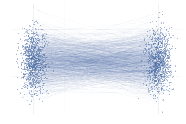
            Figure 11: Example conditional paths $\phi_t(x_0 \mid x_1)$ of \eqref{eq:g2g} with $\mu = 10$.
        </p>
    
</div>

        </div>
</div>
    </div>

    <p>In the end, we’re really just interested in learning the <em>marginal</em> paths $\phi_t(x_0)$ for initial points $x_0$ that are probable under $p_0$, which we can then use to generate samples $x_1 = \phi_1(x_0)$. In this simple example, we can obain closed-form expressions for $\phi_t(x_0)$ corresponding to the conditional paths $\phi_t(x_0 \mid x_1)$ of \eqref{eq:g2g}, as visualised below.</p>

    <div class="my-center">
      <div>
<div class="my-image-container">

          <div class="image-container">
    <img src="/blog/assets/images/flow-matching/g2g-forward_samples-one-color.png" alt="Example marginal paths $\phi_t(x_0)$ of \eqref{eq:g2g} with $\mu = 10$." id="figure-g2g-marginal-paths-one-color" style="width: 100%; max-width: 400px" />
    
        <p class="caption">
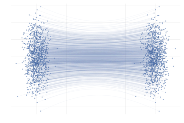
            Figure 12: Example marginal paths $\phi_t(x_0)$ of \eqref{eq:g2g} with $\mu = 10$.
        </p>
    
</div>

        </div>
</div>
    </div>

    <p>With that in mind, let’s pick a random initial point $x_0$ from $p_0$, and then compare a MC estimator for $u_t(x_0)$ at different values of $t$ along the path $\phi_t(x_0)$, i.e. we’ll be looking at
<!-- $$
u_t \big( \phi_t(x_0) \big) \approx \frac{1}{n} \sum_{i = 1}^n u_t \big( \phi_t(x_0) \mid x_1^{(i)} \big) \frac{p_t(\phi_t(x_0) \mid x_1^{(i)})}{p_t(\phi_t(x_0))} \quad \text{with } x_1^{(i)} \sim p_1.
$$ --></p>

\[\begin{equation*}
\begin{split}
u_t \big( \phi_t(x_0) \big) 
&amp;= \E_{p_{1 \mid t}}\left[u_t \big( \phi_t(x_0) \mid x_1 \big)\right] \\
&amp;\approx \frac{1}{n} \sum_{i = 1}^n u_t \big( \phi_t(x_0) \mid x_1^{(i)} \big) \ \text{with } x_1^{(i)} \sim p_{1 \mid t}(x_1 \mid \phi_t(x_0)).
\end{split}
\end{equation*}\]

    <p>In practice we don’t have access to the posterior \(p_{1 \mid t}(x_1 \mid x_t)\), but in this specific setting we do have closed-form expressions for everything (Albergo &amp; Vanden-Eijnden, 2022), and so we can visualise the marginal vector field \(u_t\big( \phi_t(x_0)\big)\) and the conditional vector fields \(u_t \big( \phi_t(x_0) \mid x_1^{(i)} \big)\) for all our “data” samples \(x_1^{(i)}\) and see how they compare.
This is shown in the figure below.</p>

    <div class="my-center">
      <div>

<div class="my-side-by-side">

          <div class="my-image-container">

            <div class="image-container">
    <img src="/blog/assets/images/flow-matching/g2g-vector-field-samples-with-traj-single-2.png" alt="" id="figure-g2g-vector-field-samples-with-traj-single-2.png" style="width: 100%; max-width: 400px" />
    
</div>

          </div>

          <div class="my-image-container">

            <div class="image-container">
    <img src="/blog/assets/images/flow-matching/g2g-vector-field-samples-with-traj-single-1.png" alt="" id="figure-g2g-vector-field-samples-with-traj-single-1.png" style="width: 100%; max-width: 400px" />
    
</div>

          </div>

        </div>

<div>

<p class="caption">
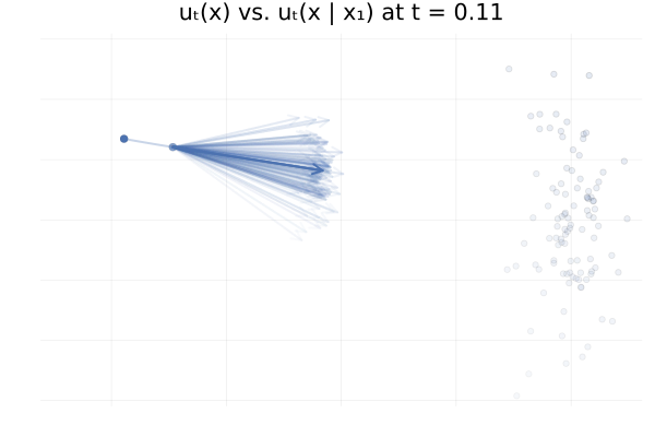
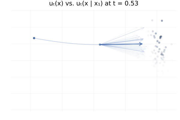
Figure 13: Marginal vector field $u_t(x)$ vs. conditional vector field $u_t(x \mid x_1)$ for samples $x_1 \sim p_1$. Here $p_0 = p_1 = \mathcal{N}(0, 1)$ and the two trajectories are according to the marginal vector field $u_t(x)$. Samples $x_1$ transparency is given by the IS weight $p_t(x \mid x_1) / p_t(x)$.
</p>
<!-- their importance weight $p_t(x \mid x_1) q(x_1) / p_t(x)$. -->

</div>

</div>
    </div>

    <!-- From the above figures, we can immediately see how for small $t$, i.e. near 0, the IS weights for the different data points $x_1^{(i)}$ are basically all the same, but as $t$ increases and get closer to 1 the estimator is dominated by only a few data samples. -->
    <p>From the above figures, we can immediately see how for small $t$, i.e. near 0, the posterior $p_{1 \mid t}(x_1 \mid x_t)$ is quite scattered so the marginalisation giving $u_t$ involves many equally likely data samples $x_1$. In contrast, when $t$ increases and get closer to 1, $p_{1 \mid t}(x_1 \mid x_t)$ gets quite concentrated over much fewer samples $x_1$.</p>

  </div>

</details>

<p>Moreover, equipped with the knowledge of \eqref{eq:cf-from-cond-vf}, we can replace</p>

\[\begin{align}
\mathcal{L}_{\mathrm{FM}}(\theta) = \mathbb{E}_{t \sim \mathcal{U}[0, 1], x \sim p_t}\left[\|
u_\theta(t, x) - u(t, x) \|^2 \right],
\end{align}\]

<p>where  $u_t(x) = \mathbb{E}_{x_1 \sim p_{1 \mid t}} \left[ u_t(x \mid x_1) \right]$, 
with an equivalent loss regressing the <em>conditional</em> vector field $u_t(x \mid x_1)$ and marginalising $x_1$ instead:</p>

\[\begin{equation*}
\mathcal{L}_{\mathrm{CFM}}(\theta) = \mathbb{E}_{t \sim \mathcal{U}[0, 1], x_1 \sim q, x_t \sim p_t(x \mid x_1)}\left[\|
u_\theta(t, x) - u_t(x \mid x_1) \|^2 \right].
\end{equation*}\]

<p>These losses are equivalent in the sense that</p>

\[\begin{equation*}
\nabla_\theta \mathcal{L}_{\mathrm{FM}}(\theta) = \nabla_\theta \mathcal{L}_{\mathrm{CFM}}(\theta),
\end{equation*}\]

<p>which implies that we can use \({\mathcal{L}}_{\text{CFM}}\) instead to train the parametric vector field $u_{\theta}$.
We defer the full proof to the footnote<sup id="fnref:CFM" role="doc-noteref"><a href="#fn:CFM" class="footnote" rel="footnote">9</a></sup>, but show the key idea below.
By developing the squared norm in both losses, we can easily show that the squared terms are equal or independent of $\theta$.
Let’s develop the inner product term for \({\mathcal{L}}_{\text{FM}}\) and show that it is equal to the inner product of \({\mathcal{L}}_{\text{CFM}}\):</p>

\[\begin{align}
\mathbb{E}_{x \sim p_t} ~\langle u_\theta(t, x), \hltwo{u_t(x)} \rangle 
&amp;= \int \langle u_\theta(t, x), \hltwo{\int} u_t(x \mid x_1) \hltwo{\frac{p_t(x \mid x_1)q(x_1)}{p_t(x)} dx_1} \rangle p_t(x) \mathrm{d} x \\
&amp;= \int \langle u_\theta(t, x), \int u_t(x \mid x_1) p_t(x \mid x_1)q(x_1) dx_1 \rangle \dd{x} \\
&amp;= \int \int \langle u_\theta(t, x), u_t(x \mid x_1) \rangle p_t(x \mid x_1)q(x_1) dx_1 \dd{x} \\
&amp;= \mathbb{E}_{q_1(x_1) p(x \mid x_1)} ~\langle u_\theta(t, x), u_t(x \mid x_1) \rangle
\end{align}\]

<p>where in the $\hltwo{\text{first highlighted step}}$ we used the expression of $u_t(x)$ in \eqref{eq:cf-from-cond-vf}.</p>

<!-- > [name=emilem] The following paragraph is key, perhaps it can be improved? -->

<p>The benefit of the CFM loss is that once we define the conditional probability path $p_t(x \mid x_1)$, we can construct an unbiased Monte Carlo estimator of the objective using samples $\big( x_1^{(i)} \big)_{i = 1}^n$ from the data target $q_1$!</p>

<p>This estimator can be efficiently computed as it involves an expectation over the joint $q_1(x_1)p_t(x \mid x_1)$ 
, of the conditional vector field $u_t (x \mid x_1)$ both being available as opposed to the marginal vector field $u_t$ which involves an expectation over the posterior $p_{1 \mid t}(x_1 \mid x)$.</p>

<!-- We also restrict to conditional paths whose vector field $u_t(x \mid x_1)$ is "simple enough" so that we can compute it in closed form. But, as we'll see, this is not too difficult to achieve. -->

<p>We note that, as opposed to the log-likelihood maximisation loss of CNFs which does not put any preference over which vector field $u_t$ can be learned, the CFM loss does specify one via the choice of a conditional vector field, which will be regressed by the neural vector field $u_\theta$.</p>

<!--

To do so we construct a _probability path_ $p_t$ which interpolates between the reference (i.e. noise) distribution $q_0$ and the data distribution $q_1$, i.e. $p_{t=0}=q_0$ and $p_{t=1}=q_1 * \mathrm{N}(0, \sigma^2)$.

Lipman et al. (2023) achieves this by constructing $p_t$ as mixture of simpler probability paths: $p_t \triangleq \int p_t(\cdot \mid x_1) q_1(x_1) \dd{x}_1$, via a _conditional probability path_ $p_t(\cdot \mid x_1)$ satisfying $p_1(\cdot \mid x_1)=\mathrm{N}(x_1, \sigma^2) \xrightarrow[\sigma \rightarrow 0]{} \delta_{x_1}$ and $p_0(\cdot \mid x_1)=p_0$.

As a result both endpoints constraint are satisfied since ones recovers
- at $t=1$ the data distribution $p_1(x) = \int p_1(x \mid x_1) q_1(x_1) \dd{x}_1 = \int \mathrm{N}(x_1, \sigma^2) q_1(x_1) \dd{x}_1 \xrightarrow[\sigma \rightarrow 0]{} q_1(x)$
- at $t=0$ the reference distribution $p_0(x) = \int p_0(x \mid x_1) q_1(x_1) \dd{x}_1 = \int q_0(x) q_1(x_1) \dd{x}_1 = q_0(x)$.

<div markdown="1" style="display: flex; margin-top:-0px; margin-bottom:-0px;">
<div markdown="1" style="margin: auto;">

![cond_ut](https://hackmd.io/_uploads/HyLrNEWSa.jpg =200x)
</div>
</div>

We have defined a probability path $p_t$ in terms of conditional probability path $p_t(\cdot \mid x_1)$, yet how do we define the latter?
We know that the transport equation $\frac{\partial}{\partial_t} p_t(x_t) = - (\nabla \cdot (u_t p_t))(x_t)$ relates a vector field (i.e. vector field) to a propability path $p_t$ (given an initial value $p_{t=0} = q_0$).
As such it is sufficient to construct a _conditional vector field_ $u_t(\cdot \mid x_1)$ which induces a conditional probability path $p_t(\cdot \mid x_1)$ with the right boundary conditions.

-->

<h3 id="gaussian-probability-paths">Gaussian probability paths</h3>
<p>Let’s now look at practical example of conditional vector field and the corresponding probability path. Suppose we want conditional vector field which generates a path of Gaussians, i.e.</p>

\[\begin{equation*}
p_t(x \mid x_1) = \mathcal{N}(x; \mu_t(x_1), \sigma_t(x_1)^2 \mathrm{I})
\end{equation*}\]

<p>for some mean $\mu_t(x_1)$ and standard deviation $\sigma_t(x_1)$.</p>

<!-- This means one can sample $x_t \mid x_1 ~ p_t(\cdot \mid x_1)$ as $x_t = \phi(x_0 \mid x_1)$ with $\phi(x \mid x_1) = \sigma_t(x_1) x + \mu_t(x_1)$ and $x_0 \sim \mathcal{N}(0, \mathrm{I})$. -->
<!--  -->
<p>One conditional vector field inducing the above-defined conditional probability path is given by the following expression:</p>

\[\begin{equation}
\label{eq:gaussian-path}
u_t(x \mid x_1) = \frac{\dot{\sigma_t}(x_1)}{\sigma_t(x_1)} (x - \mu_t(x_1)) + \dot{\mu_t}(x_1)
\end{equation}\]

<p>as shown in the proof below.</p>

<details class="my-proof my-box">
<summary>Proof</summary>

We have

$$
\begin{equation*}
\phi_t(x \mid x_1) = \mu_t(x_1) + \sigma_t(x_1) x
\end{equation*}
$$

and we want to determine $u_t(x \mid x_1)$ such that

$$
\begin{equation*}
\frac{\dd}{\dd t} \phi_t(x) = u_t \big( \phi_t(x) \mid x_1 \big)
\end{equation*}
$$

First note that the LHS is

$$
\begin{equation*}
\begin{split}
\frac{\dd{}}{\dd{} t} \phi_t(x) &amp;= \frac{\dd{}}{\dd{} t} \bigg( \mu_t(x_1) + \sigma_t(x_1) x \bigg) \\
&amp;= \dot{\mu_t}(x_1) + \dot{\sigma_t}(x_1) x
\end{split}
\end{equation*}
$$

so we have

$$
\begin{equation*}
\dot{\mu_t}(x_1) + \dot{\sigma_t}(x_1) x = u_1 \big( \phi_t(x \mid x_1) \mid x_1 \big)
\end{equation*}
$$

Suppose that $u_1$ is of the form

$$
\begin{equation*}
u_1\big( \phi_t(x) \mid x_1\big) = h\big(t, \phi_t(x), x_1\big) \dot{\mu_t}(x_1) + g\big(t, \phi_t(x), x_1\big) \dot{\sigma_t}(x_1)
\end{equation*}
$$

for some functions $h$ and $g$.
Reading of the components from the previous equation, we then see that we require

$$
\begin{equation*}
h\big(t, \phi_t(x), x_1\big) = 1 \quad \text{and} \quad
g(t, \phi_t(x), x_1) = x
\end{equation*}
$$

The simplest solution to the above is then just

$$
\begin{equation*}
h(t, x, x_1) = 1
\end{equation*}
$$

i.e. constant function, and

$$
\begin{equation*}
g(t, x, x_1) = \phi_t^{-1}(x) = \frac{x - \mu_t(x_1)}{\sigma_t(x_1)}
\end{equation*}
$$

such that

$$
\begin{equation*}
g\big(t, \phi_t(x), x_1) = \phi_t^{-1} \big( \phi_t(x) \big) = x
\end{equation*}
$$

resulting in

$$
\begin{equation*}
u_t \big( x \mid x_1 \big) = \dot{\mu_t}(x_1) + \dot{\sigma_t}(x_1) \bigg( \frac{x - \mu_t(x_1)}{\sigma_t(x_1)} \bigg)
\end{equation*}
$$

as claimed.

</details>

<!-- Example begin -->
<details class="my-success my-box" id="example-linear-interpolation" open="true">
  <summary>
Example: Linear interpolation
</summary>

  <div>

    <p>A simple choice for the mean $\mu_t(x_1)$ and std. $\sigma_t(x_1)$ is the linear interpolation for both, i.e.</p>

\[\begin{align*}
\hlone{\mu_t(x_1)} &amp;\triangleq t x_1 \quad &amp;\text{and} \quad \hlthree{\sigma_t(x_1)} &amp;\triangleq (1 - t) + t \sigmamin \\
\hltwo{\dot{\mu}_t(x_1)} &amp;\triangleq x_1 \quad &amp;\text{and} \quad \hlfour{\dot{\sigma}_t(x_1)} &amp;\triangleq -1 + \sigmamin
\end{align*}\]

    <p>so that</p>

\[\begin{equation*}
\big( {\hlone{\mu_0(x_1)}} + {\hlthree{\sigma_0(x_1)}} x_1 \big) \sim p_0 \quad \text{and} \quad \big( {\hlone{\mu_1(x_1)}} + {\hlthree{\sigma_1(x_1)}} x_1 \big) \sim \mathcal{N}(x_1, \sigmamin^2 I)
\end{equation*}\]

    <!-- and so -->
    <!-- $$ -->
    <!-- p_t(x \mid x_1) = \mathcal{N}\big(x; t x_1, (1 - t) + t \sigmamin \big) -->
    <!-- $$ -->

    <p>In addition, letting $p_0 = \mathcal{N}([-\mu, 0], I)$ and $p_1 = \mathcal{N}([+\mu, 0], I)$ for some $\mu &gt; 0$, we’re back to the \ref{eq:g2g} example from earlier.</p>

    <p>We can then plug this choice of $\mu_t(x_1)$ and $\sigma_t(x_1)$ into \eqref{eq:gaussian-path} to obtain the conditional vector field, writing $\hlthree{\sigma_t(x_1)} = 1 - (1 - \sigmamin) t$ to make our lives simpler,</p>

\[\begin{equation*}
\begin{split}
u_t(x \mid x_1) &amp;= \frac{\hlfour{- (1 - \sigmamin)}}{\hlthree{1 - (1 - \sigmamin) t}} (x - \hlone{t x_1}) + \hltwo{x_1} \\
&amp;= \frac{1}{(1 - t) + t \sigmamin} \bigg( - (1 - \sigmamin) (x - t x_1) + \big(1 - (1 - \sigmamin) t \big) x_1 \bigg) \\
&amp;= \frac{1}{(1 - t) + t \sigmamin} \bigg( - (1 - \sigmamin) x + x_1 \bigg) \\
&amp;= \frac{x_1 - (1 - \sigmamin) x}{1 - (1 - \sigmamin) t}.
\end{split}
\end{equation*}\]

    <p>Below you can see the difference between $\phi_t(x_0)$ (top figure) and $\phi_t(x_0 \mid x_1)$ (bottom figure) for pairs $(x_0, x_1)$ with $x_0 \sim p_0$ and $x_1 = \phi_t(x_0)$. The paths are coloured by the sign of the 2nd vector component of $x_0$ to more clearly highlight the difference between the marginal and conditional flows.</p>

    <div class="my-center">
      <div>
<div class="my-side-by-side">

          <div class="my-image-container">

            <div class="image-container">
    <img src="/blog/assets/images/flow-matching/g2g-vector-field-samples-cond.png" alt="Realizations of paths from $p_0$ to $p_1$ following conditional vector fields $u_t(x \mid x_1)$. Paths are highlighted by the sign of the 2nd vector component at time $t=1$." id="figure-g2g-vector-field-samples-cond.png" style="width: 100%; max-width: 400px" />
    
        <p class="caption">
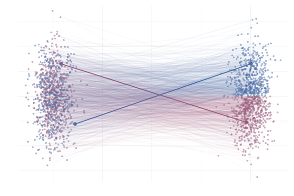
            Figure 14: Realizations of paths from $p_0$ to $p_1$ following conditional vector fields $u_t(x \mid x_1)$. Paths are highlighted by the sign of the 2nd vector component at time $t=1$.
        </p>
    
</div>

          </div>

          <div class="my-image-container">

            <div class="image-container">
    <img src="/blog/assets/images/flow-matching/g2g-forward_samples.png" alt="Paths from $p_0$ to $p_1$ following the true marginal vector field $u_t(x)$. Paths are highlighted by the sign of the 2nd vector component." id="figure-g2g-forward_samples.png" style="width: 100%; max-width: 400px" />
    
        <p class="caption">
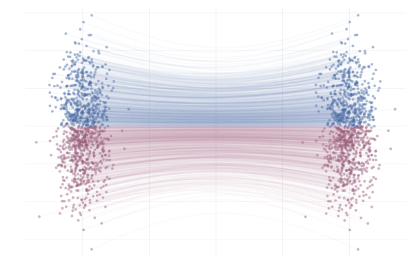
            Figure 15: Paths from $p_0$ to $p_1$ following the true marginal vector field $u_t(x)$. Paths are highlighted by the sign of the 2nd vector component.
        </p>
    
</div>

          </div>

        </div>
</div>
    </div>

  </div>

</details>

<!-- Example end -->

<!-- 
<div markdown="1" class="my-success my-box">
The _conditional_ vector field is the OT map!
</div>
<div markdown="1" class="my-warning my-box">
Does not guarantee that the _marginal_ vector field is the OT map!
</div>
-->

<!-- 

## Gaussian probability paths (Cont'd)

:::danger
remove diffusion vf
</div>
### (conditional) diffusion vf
- $dx_t = -\frac{1}{2}\sqrt{\beta(t)} x_t \dd{t} + \beta(t) \dd{B}_t$
- $\alpha_t = e^{-\frac{1}{2}\int_0^t \beta(s) \dd{s}}$
- $\mu_t = \alpha_{1-t} x_1$ and $\sigma_t^2 = 1 - \alpha_{1-t}^2$
- $u_t(x \mid x_1) = -\frac{\sigma'_{1-t}}{\sigma_{1-t}}(x - x_1)$

### (conditional) OT vf
- $\mu_t = t x_1$ and $\sigma_t = 1 - t = (1 - (1 - \sigma_{\min})t$
- $u_t(x \mid x_1) = \frac{1}{1 - t}(x_1 - x) = \frac{1}{1 - (1 - \sigma_\min)t}(x_1 - (1 - \sigma_\min)x)$
<div markdown="1" class="my-warning my-box">
Does not guarantee that the _marginal_ vector field is the OT map!
</div>

-->

<h3 id="but-is-cfm-really-all-rainbows-and-unicorns">But is CFM really all rainbows and unicorns?</h3>

<!-- > [name=emilem] Perhaps this is a bit dramatic as FM already works well witout mini batch OT? -->

<p>Unfortunately not, no. There are two issues arising from <em>crossing conditional paths</em>. We will explain this just after, but now we stress that this leads to</p>
<ol>
  <li>Non-straight marginal paths $\Rightarrow$ ODE hard to integrate $\Rightarrow$ slow sampling at inference.</li>
  <li>Many possible $x_1$ for a noised $x_t$ $\Rightarrow$ high CFM loss variance $\Rightarrow$ slow training convergence.</li>
</ol>

<p>To get a better understanding of what these two points above, let’s revisit the \ref{eq:g2g} example once more. As we see in the figures below, realizations of the conditional vector field $u_t(x \mid x_1)$, i.e. sampling from the process</p>

\[\begin{equation*}
\begin{split}
x_1 &amp; \sim q \\
x_t &amp; \triangleq \phi_t(x \mid x_1)
\end{split}
\end{equation*}\]

<p>result in paths that are quite different from the marginal paths as illustrated in the figures below.</p>

<!-- > [name=emilem]  Gausian to gausian example instead -->

<div class="my-center">
  <div>
<div class="my-side-by-side">

      <div>
<div class="my-image-container">

          <div class="image-container">
    <img src="/blog/assets/images/flow-matching/g2g-vector-field-samples-cond.png" alt="Realizations of conditional paths from $p_0 = p_1 = \mathcal{N}(0, 1)$ for two different $x_1^{(i)}, x_1^{(2)} \sim q$ with conditional vector field given by $u_t(x \mid x_1) = (1 - t) x + t x_1$." id="figure-.png" style="width: 100%; max-width: 400px" />
    
        <p class="caption">
            Figure 16: Realizations of conditional paths from $p_0 = p_1 = \mathcal{N}(0, 1)$ for two different $x_1^{(i)}, x_1^{(2)} \sim q$ with conditional vector field given by $u_t(x \mid x_1) = (1 - t) x + t x_1$.
        </p>
    
</div>

          <!-- ![forward_samples](https://hackmd.io/_uploads/r1skZ4CI6.png) -->

        </div>
</div>

      <div>
<div class="my-image-container">

          <div class="image-container">
    <img src="/blog/assets/images/flow-matching/g2g-forward_samples.png" alt="Paths from $p_0$ to $p_1$ following the true marginal vector field $u_t(x)$. Paths are highlighted by the sign of the 2nd vector component." id="figure-.png" style="width: 100%; max-width: 400px" />
    
        <p class="caption">
            Figure 17: Paths from $p_0$ to $p_1$ following the true marginal vector field $u_t(x)$. Paths are highlighted by the sign of the 2nd vector component.
        </p>
    
</div>

          <!-- ![forward_samples](https://hackmd.io/_uploads/H1hVWVAUa.png) -->

        </div>
</div>

    </div>
</div>
</div>

<p>In particular, we can see that the marginal paths $\phi_t(x)$ <em>do not cross</em>; this is indeed just the uniqueness property of ODE solutions. A realization of the conditional vector field $u_t(x \mid x_1)$ also exhibits the “non-crossing paths” property, similar to the marginal flows $\phi_t(x)$, however paths $\phi_t(x \mid x_1)$ corresponding to <em>different</em> realizations $x_1 \sim q_1$ may intersect, as highlighted in the figure above.</p>

<!-- > [name=emilem] I like this bit but would the argument be more straightforward if $\hlone{x_t^{(1)}} = \hlone{x_t^{(2)}}$ ? -->

<p>Consider two highlighted paths in the visualization of $u_t(x \mid x_1)$, with data samples $\hlone{x_1^{(1)}}$ and $\hlthree{x_1^{(2)}}$. When learning a parameterized vector field $u_{\theta}(t, x)$ via stochastic gradient descent (SGD), we approximate the CFM loss as:</p>

\[\mathcal{L}_{\mathrm{CFM}}(\theta) \approx \frac{1}{2} \norm{u_{\theta}(t, \hlone{x_t^{(1)}}) - u(t, \hlone{x_t^{(1)}} \mid \hlone{x_1^{(1)}})} + \frac{1}{2} \norm{u_{\theta}(t, \hlthree{x_t^{(2)}}) - u(t, \hlthree{x_t^{(2)}} \mid \hlthree{x_1^{(2)}})}\]

<p>where $t \sim \mathcal{U}[0, 1]$, $\hlone{x_1^{(1)}}, \hlthree{x_1^{(2)}} \sim q_1$, and $\hlone{x_t^{(1)}} \sim p_t(\cdot \mid \hlone{x_1^{(1)}}), \hlthree{x_t^{(2)}} \sim p_t(\cdot \mid \hlthree{x_1^{(2)}})$. We compute the gradient with respect to $\theta$ for a gradient step.</p>

<p>In such a scenario, we’re attempting to align $u_{\theta}(t, x)$ with two different vector fields whose corresponding paths are impossible under the marginal vector field $u(t, x)$ that we’re trying to learn! This fact can lead to increased variance in the gradient estimate, and thus slower convergence.</p>

<p>In slightly more complex scenarios, the situation becomes even more striking. Below we see a nice example from Liu et al. (2022) where our reference and target are two different mixture of Gaussians in 2D differing only by the sign of the mean in the x-component. Specifically,</p>

\[\begin{equation}
\tag{MoG-to-MoG}
\label{eq:mog2mog}
\begin{split}
p_{\hlone{0}} &amp;= (1 / 2)\mathcal{N}([{\hlone{-\mu}}, -\mu], I) + (1 / 2) \mathcal{N}([{\hlone{-\mu}}, +\mu], I) \\
\text{and} \quad p_{\hltwo{1}} &amp;= (1 / 2) \mathcal{N}([{\hltwo{+\mu}}, -\mu], I) + (1 / 2) \mathcal{N}([{\hltwo{+\mu}}, +\mu], I) \\
\text{with} \quad \phi_t(x_0 \mid x_1) &amp;= (1 - t) x_0 + t x_1
\end{split}
\end{equation}\]

<p>where we set $\mu = 10$, unless otherwise specified.</p>

<div class="my-center">
  <div>
<div class="my-side-by-side">

      <div class="my-image-container">

        <div class="image-container">
    <img src="/blog/assets/images/flow-matching/vector-field-samples-cond.png" alt="Realizations of conditional paths following conditional vector field $u_t(x \mid x_1)$ from \eqref{eq:mog2mog}. Paths are highlighted by the sign of the 2nd vector component." id="figure-vector-field-samples-cond.png" style="width: 100%; max-width: 400px" />
    
        <p class="caption">
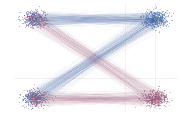
            Figure 18: Realizations of conditional paths following conditional vector field $u_t(x \mid x_1)$ from \eqref{eq:mog2mog}. Paths are highlighted by the sign of the 2nd vector component.
        </p>
    
</div>

        <!-- ![vector-field-samples-cond](https://hackmd.io/_uploads/SyG9OF_IT.png) -->
      </div>

      <div class="my-image-container">

        <div class="image-container">
    <img src="/blog/assets/images/flow-matching/vector-field-samples-marginal.png" alt="Realizations of marginal paths following the marginal vector field $u_t(x)$ from \eqref{eq:mog2mog}. Paths are highlighted by the sign of the 2nd vector component." id="figure-vector-field-samples-marginal.png" style="width: 100%; max-width: 400px" />
    
        <p class="caption">
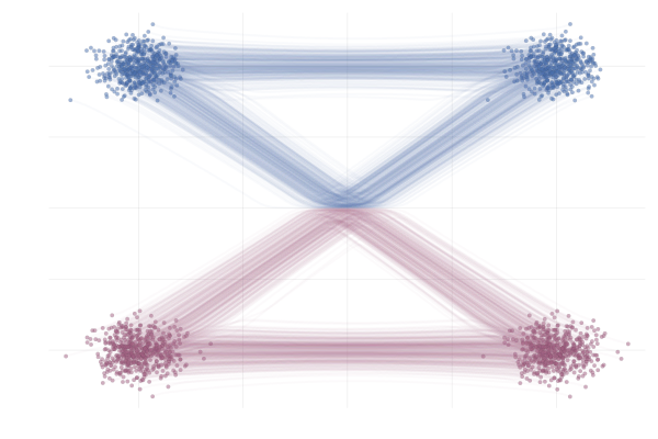
            Figure 19: Realizations of marginal paths following the marginal vector field $u_t(x)$ from \eqref{eq:mog2mog}. Paths are highlighted by the sign of the 2nd vector component.
        </p>
    
</div>

        <!-- ![forward_samples](https://hackmd.io/_uploads/SJusOFuL6.png) -->
      </div>

    </div>
</div>
</div>

<p>Here we see that marginal paths (bottom figure) end up looking <em>very</em> different from the conditional paths (top figure). Indeed, at training time paths may intersect, whilst at sampling time they cannot (due to the uniqueness of the ODE solution). As such we see on the bottom plot that some (marginal) paths are quite curved and would therefore require a greater number of discretisation steps from the ODE solver during inference.</p>

<p>We can also see how this leads to a significant variance of the CFM loss estimate for $t \approx 0.5$ in the figure below.
More generally, samples from the reference distribution which are arbitrarily close to eachothers can be associated with either target modes, leading to high variance in the vector field regression loss.</p>

<div class="my-center">
  <div>
<div class="my-side-by-side">

      <div class="my-image-container">

        <div class="image-container">
    <img src="/blog/assets/images/flow-matching/vector-field-samples-with-traj.png" alt="Realizations of conditional paths $\phi_t(x_0 \mid x_1)$ following the conditional vector field $u_t(x \mid x_1)$ for \eqref{eq:mog2mog}." id="figure-vector-field-samples-with-traj.png" style="width: 100%; max-width: 400px" />
    
        <p class="caption">
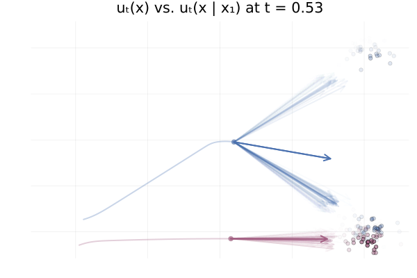
            Figure 20: Realizations of conditional paths $\phi_t(x_0 \mid x_1)$ following the conditional vector field $u_t(x \mid x_1)$ for \eqref{eq:mog2mog}.
        </p>
    
</div>

        <!-- ![vector-field-samples-with-traj](https://hackmd.io/_uploads/B1Vuz4ALa.png) -->

      </div>

      <div class="my-image-container">

        <div class="image-container">
    <img src="/blog/assets/images/flow-matching/variance_cond_vector_field.png" alt="Variance of conditional vector field over $p_{1 \mid t}$ for both blue and red trajectories for \eqref{eq:mog2mog}." id="figure-variance_cond_vector_field.png" style="width: 100%; max-width: 400px" />
    
        <p class="caption">
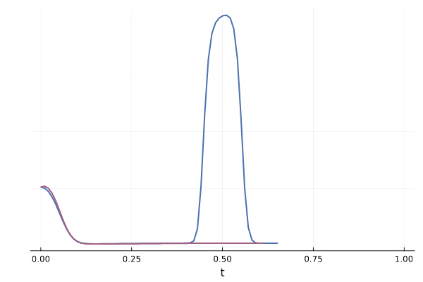
            Figure 21: Variance of conditional vector field over $p_{1 \mid t}$ for both blue and red trajectories for \eqref{eq:mog2mog}.
        </p>
    
</div>

        <!-- ![variance_cond_vector_field](https://hackmd.io/_uploads/r1XcxLmPa.png) -->

      </div>

    </div>
</div>
</div>

<p>An intuitive solution would be to associate data samples with reference samples which are close instead of some arbitrary pairing.
We’ll detail this idea next via the concept of couplings and optimal transport.
<!-- To alleviate this issue, we'll turn to couplings and optimal transport. --></p>

<!-- 
#### Crossing paths

Let's observe in the following plot, the toy setting where both the data and noise distribution are bimodal mixtures. On the LHS, we can see possible linear interpolations between samples $x_1,x_0 \sim q(x_1,x_0) = q_1(x_1) q_0(x_0)$, as given by the conditional vector field. On the RHS we see different paths from the learnt flow $\dd x_t = u_\theta(t, x_t) \dd t$. For a well defined ODE--assuming continuous and Lipschitz vector field, solutions exist and are unique, and as such paths _cannot cross each other_ at any time $t$.
As a consequence the paths are different at training and inference time.
There are two immediate consequences:
1. At inference time, the paths aren't as 'straight' as they were if closer modes where 'matched' together, leading to an unnecessarily high number of discretisation steps (for a given error threshold).
2. At training time, noise samples which are arbitrarily close by can be associated with either data modes, and as such lead to high variance in the vector field regression loss.


<div markdown="1" class="my-center">
<div>
<div markdown="1" class="my-side-by-side">
<div markdown="1" class="my-image-container">

![forward_samples](https://hackmd.io/_uploads/SyG9OF_IT.png)
*Interpolation path $\phi(x_t \mid x_0,x_1)$*.

</div>
<div markdown="1" class="my-image-container">

![forward_samples](https://hackmd.io/_uploads/SJusOFuL6.png)
*Inference path $\phi(x_t \mid x_0)$*.

</div>
</div>
<div>

Figure: *Independent coupling $q(x_0, x_1) = q(x_0)q(x_1)$.*

</div>
</div>
</div>

<!--  -->
<!-- <div markdown="1" style="display: flex; margin-top:-10px; margin-bottom:-10px;">
<div markdown="1" style="margin: auto;">

![cond_ut](https://hackmd.io/_uploads/H1_jkEjB6.jpg =400x)
</div>
</div>
 -->

<h3 id="coupling">Coupling</h3>

<p>So far we have constructed the vector field $u_t$ by conditioning and marginalising over data points $x_1$. This is referred to as a <em>one-sided conditioning</em>, where the probability path is constructed by marginalising over $z=x_1$:</p>

\[p_t(x_t) = \int p_t(x_t \mid z) q(z) \dd{z} = \int p_t(x_t \mid x_1) q(x_1) \dd{x_1}\]

<p>e.g. 
\(p(x_t  \mid  x_1) = \mathcal{N}(x_t \mid x_1, (1-t)^2)\).</p>

<div class="my-center">
  <div>
<div class="my-image-container">

      <div class="image-container">
    <img src="/blog/assets/images/flow-matching/albergo_one_sided.jpg" alt="One sided interpolation. Source: Figure (2) in Albergo &amp; Vanden-Eijnden (2022)." id="figure-albergo_one_sided.jpg" style="width: 100%; max-width: 800px" />
    
        <p class="caption">
            Figure 22: One sided interpolation. Source: Figure (2) in Albergo &amp; Vanden-Eijnden (2022).
        </p>
    
</div>

    </div>
</div>
</div>

<p>Yet, more generally, we can consider conditioning and marginalising over latent variables $z$, and minimising the following loss:</p>

\[\mathcal{L}_{\mathrm{CFM}}(\theta) = \mathbb{E}_{(t,z,x_t) \sim \mathcal{U}[0,1] q(z) p(\cdot \mid z)}[\| u_\theta(t, x_t) - u_t(x_t \mid z)\|^2].\]

<p>As suggested in Liu et al. (2023), Tong et al. (2023), Albergo &amp; Vanden-Eijnden (2022) and Pooladian et al. (2023) one can condition on <em>both</em> endpoints $z=(x_1, x_0)$ of the process, referred as <em>two-sided conditioning</em>. The marginal probability path is defined as:</p>

\[p_t(x_t) = \int p_t(x_t \mid z) q(z) \dd{z} = \int p_t(x_t \mid x_1, x_0) q(x_1, x_0) \dd{x_1} \dd{x_0}.\]

<div class="my-info my-box">

  <p>The following boundary condition on $p_t(x_t \mid x_1, x_0)$: $p_0(\cdot \mid x_1, x_0)=\delta_{x_0}$ and $p_1(\cdot \mid x_1, x_0) = \delta_{x_1}$ is required so that the marginal has the proper conditions $p_0 = q_0$ and $p_1 = q_1$.</p>

</div>

<p>For instance, a deterministic linear interpolation gives $p(x_t \mid x_0, x_1) = \delta_{(1-t)} x_0 + t x_1(x_t)$ and the simplest choice regarding the coupling $z = (x_1, x_0)$ is to consider independent samples: $q(x_1, x_0) = q_1(x_1) q_0(x_0)$.</p>

<div class="my-center">
  <div>
<div class="my-image-container">

      <div class="image-container">
    <img src="/blog/assets/images/flow-matching/albergo_two_sided.jpg" alt="Two sided interpolation. Source: Figure (2) in Albergo &amp; Vanden-Eijnden (2022)." id="figure-albergo_two_sided.jpg" style="width: 100%; max-width: 800px" />
    
        <p class="caption">
            Figure 23: Two sided interpolation. Source: Figure (2) in Albergo &amp; Vanden-Eijnden (2022).
        </p>
    
</div>

    </div>
</div>
</div>

<p>One main advantage is that this allows for non Gaussian reference distribution $q_0$.
Choosing a standard normal as noise distribution $q(x_0) = \mathcal{N}(0, \mathrm{I})$ we recover the same <em>one-sided</em> conditional probability path as earlier:</p>

\[p(x_t \mid x_1) = \int p(x_t \mid x_0, x_1) q(x_0) \dd{x_0} = \mathcal{N}(x_t \mid tx_1, (1-t)^2).\]

<!-- - $p(x_0, x_1) = p(x_0) p(x_1)$
    - $p(x_0) = \N(0, \Id)$
    - $p(x_0)$ non Gaussian
 -->

<h4 class="no_toc" id="optimal-transport-ot-coupling">Optimal Transport (OT) coupling</h4>

<!-- [Liu et al., 2022, Tong et al., 2023] suggest to alleviate this by using a **joint coupling** $q(x_1, x_0) \neq q_1(x_1) q_0(x_0)$ which correlates pairs $(x_1, x_0)$. -->
<p>Now let’s go back to the idea of <em>not</em> using an independent coupling (i.e. pairing) but instead to correlate pairs $(x_1, x_0)$ with a joint $q(x_1, x_0) \neq q_1(x_1) q_0(x_0)$.
Tong et al. (2023) and Pooladian et al. (2023) suggest using the <em>optimal transport coupling</em></p>

\[\begin{equation}
\tag{OT}
\label{eq:ot}
q(x_1, x_0) = \pi(x_1, x_0) \in \arg\inf_{\pi \in \Pi} \int \|x_1 - x_0\|_2^2 \mathrm{d} \pi(x_1, x_0)
\end{equation}\]

<p>which minimises the optimal transport (i.e. Wasserstein) cost (Monge, 1781, Peyré and Cuturi 2020).
The OT coupling $\pi$ associates samples $x_0$ and $x_1$ such that the total distance is minimised.
<!-- This prevents the crossing paths behaviour that we highlighted earlier, as permuting samples would yield non crossing paths which would have a lower total distance cost, and as such the coupling yielding to crossing paths cannot be the OT coupling. --></p>

<p>This OT coupling is illustrated in the right hand side of the figure below, adapted from Tong et al. (2023). In contrast to the middle figure which an independent coupling, the OT one does not have paths that cross. This leads to lower training variance and faster sampling<sup id="fnref:OT" role="doc-noteref"><a href="#fn:OT" class="footnote" rel="footnote">10</a></sup>.</p>

<div class="my-center">
  <div>
<div class="my-side-by-side">

      <div class="my-image-container">

        <div class="image-container">
    <img src="/blog/assets/images/flow-matching/trajectory-marginals-vertical.png" alt="One-sided conditioning (Lipman et al., 2022)" id="figure-trajectory-marginals-vertical.png" />
    
        <p class="caption">
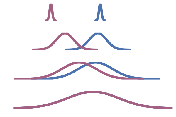
            Figure 24: One-sided conditioning (Lipman et al., 2022)
        </p>
    
</div>

      </div>

      <div class="my-image-container">

        <div class="image-container">
    <img src="/blog/assets/images/flow-matching/trajectory-marginals-vertical-cond.png" alt="Two-sided conditioning (Tong et al., 2023)" id="figure-trajectory-marginals-vertical-cond.png" />
    
        <p class="caption">
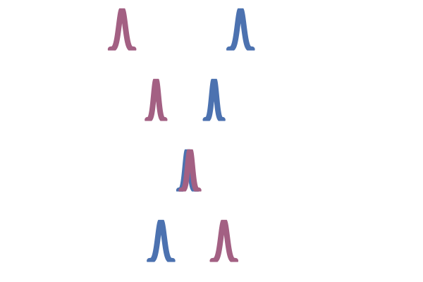
            Figure 25: Two-sided conditioning (Tong et al., 2023)
        </p>
    
</div>

      </div>

      <div class="my-image-container">

        <div class="image-container">
    <img src="/blog/assets/images/flow-matching/trajectory-marginals-vertical-ot.png" alt="OT coupling (Tong et al., 2023)" id="figure-trajectory-marginals-vertical-ot.png" />
    
        <p class="caption">
            Figure 26: OT coupling (Tong et al., 2023)
        </p>
    
</div>

      </div>

    </div>
</div>
</div>

<!--
|     |     |     |
| :-: | :-: | :-: |
|  <sub><sup>One sided</sup></sub>   |  <sub><sup>Two sided</sup></sub>   |   <sub><sup>OT</sup></sub>  |
| <img src="https://hackmd.io/_uploads/HyLrNEWSa.jpg" width="60%"> | <img src="https://hackmd.io/_uploads/S10jNNZH6.jpg" width="60%"> | <img src="https://hackmd.io/_uploads/rJ7nENbrp.jpg" width="60%"> |
 -->

<p>In practice, we cannot compute the optimal coupling $\pi$ between $x_1 \sim q_1$ and $x_0 \sim q_0$, as algorithms solving this problem are only known for finite distributions.
In fact, finding a map from $q_0$ to $q_1$ is the generative modelling problem that we are trying to solve in the first place!</p>

<p>Tong et al. (2023) and Pooladian et al. (2023) propose to approximate the OT coupling $\pi$ by computing such optimal coupling only over each mini-batch of data and noise samples, coined <strong>mini-batch OT</strong> (Fatras et al., 2020). This is scalable as for finite collection of samples the OT problem can be computed with quadratic complexity via the Sinkhorn algorithm (Peyre and Cuturi, 2020). This results in a <em>joint</em> distribution $\gamma(i, j)$ over “inputs” \(\big(x_0^{(i)}\big)_{i=1,\dots,B}\) and “outputs” \(\big(x_1^{(j)}\big)_{j=1,\dots,B}\) such that the expected distance is (approximately) minimised.  Finally, to construct a mini-batch from this $\gamma$ which we can subsequently use for training, we can either compute the expectation wrt. $\gamma(i, j)$ by considering all $n^2$ pairs (in practice, this can often boil down to only needing to consider $n$ disjoint pairs<sup id="fnref:mini-batch-ot-deterministic-vs-stochastic" role="doc-noteref"><a href="#fn:mini-batch-ot-deterministic-vs-stochastic" class="footnote" rel="footnote">11</a></sup>) or sample a new collection of training pairs $(x_0^{(i’)}, x_1^{(j’)})$ with $(i’, j’) \sim \gamma$<sup id="fnref:mini-batch-ot-sampling-size" role="doc-noteref"><a href="#fn:mini-batch-ot-sampling-size" class="footnote" rel="footnote">12</a></sup>.</p>

<p>For example, we can apply this to the \eqref{eq:g2g} example from before, which almost completely removes the crossing paths behaviour described earlier, as can be seen in the figure below.</p>

<div class="my-center">
  <div>

<div class="my-side-by-side">

      <div class="my-image-container">

        <div class="image-container">
    <img src="/blog/assets/images/flow-matching/g2g-cond-paths-one-color.png" alt="" id="figure-g2g-cond-paths-one-color--ot" style="width: 100%; max-width: 400px" />
    
</div>

      </div>

      <div class="my-image-container">

        <div class="image-container">
    <img src="/blog/assets/images/flow-matching/g2g-cond-paths-one-color-ot.png" alt="" id="figure-g2g-cond-paths-one-color-ot--ot" style="width: 100%; max-width: 400px" />
    
</div>

      </div>

    </div>

<div>

<p class="caption">
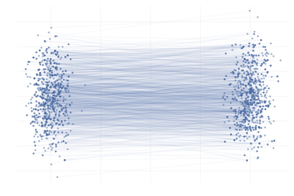
Figure 27: \eqref{eq:g2g} with uniformly sampled pairings (left) and with OT pairings (right).
</p>

</div>

</div>
</div>

<p>We also observe similar behavior when applying this the more complex example \eqref{eq:mog2mog}, as can be seen in the figure below.</p>

<div class="my-center">
  <div>

<div class="my-side-by-side">

      <div class="my-image-container">

        <div class="image-container">
    <img src="/blog/assets/images/flow-matching/mog2mog-cond-paths-one-color.png" alt="" id="figure-g2g-cond-paths-one-color--ot" style="width: 100%; max-width: 400px" />
    
</div>

      </div>

      <div class="my-image-container">

        <div class="image-container">
    <img src="/blog/assets/images/flow-matching/mog2mog-cond-paths-one-color-ot.png" alt="" id="figure-g2g-cond-paths-one-color-ot--ot" style="width: 100%; max-width: 400px" />
    
</div>

      </div>

    </div>

<div>

<p class="caption">
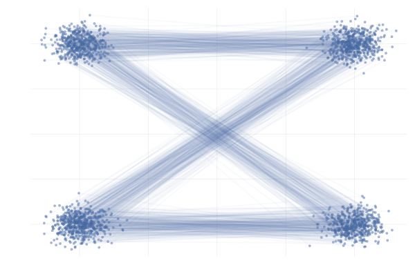
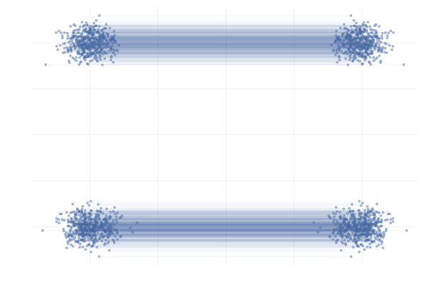
Figure 28: \eqref{eq:mog2mog} with uniformly sampled pairings (left) and with OT pairings (right).
</p>

</div>

</div>
</div>

<p>All in all, making use of mini-batch OT seems to be a strict improvement over the uniform sampling approach to constructing the mini-batch in the above examples and has been shown to improve practical performance in a wide range of applications (Tong et al., 2023; Klein et al., 2023).</p>

<p>It’s worth noting that in \eqref{eq:ot} we only considered choosing the coupling $\gamma(i, j)$ such that we minimize the expected squared Euclidean distance. This works well in the examples \eqref{eq:g2g} and \eqref{eq:mog2mog}, but we could also replace squared Euclidean distance with some other distance metric when constructing the coupling $\gamma(i, j)$. For example, if we were modeling molecules using CNFs, it might also make sense to pick $(i, j)$ such that $x_0^{(i)}$ and $x_1^{(j)}$ are also rotationally aligned as is done in the work of Klein et al. (2023).</p>

<!-- > [name=Tor] Should probably have some plots or something from the paper here to demonstrate that minibtach OT is worth it. -->
<!-- > [name=emilem] I agree, I'd suggest  -->

<h1 id="quick-summary">Quick Summary</h1>

<!-- > [name=Tor] Maybe we should have a slightly more informal tone here? And
> - Maybe mention some open-source impls if people want to get started (unless we cook up something) on their own? -->

<p>In short, we’ve shown that flow matching is an efficient approach to training continuous normalising flows (CNFs), by directly regressing over the vector field instead of explicitly training by maximum likelihood.
This is enabled by constructing the target vector field as the marginalisation of simple conditional vector fields which (marginally) interpolate between the reference and data distribution, but crucially for which we can evaluate and integrate over time.
A neural network parameterising the vector field can then be trained by regressing over these conditional vector fields.
Similarly to CNFs, samples can be obtained at inference time by solving the ODE associated with the neural vector field.</p>

<!-- which bridge between a noise refence distribution and a target data distribution, and as such constructs a generative model. -->

<p>In this post we have not talked about diffusion (i.e. score based) models on purpose as they are not necessary for understanding flow matching.
Yet these are deeply related and even exactly the same in some settings.
We are planning to explore these connections, along with generalisations in a follow-up post!</p>

<h1 id="citation">Citation</h1>

<p>Please cite us as:</p>

<div class="language-plaintext highlighter-rouge"><div class="highlight"><pre class="highlight"><code>@misc{mathieu2024flow,
  title   = "An Introduction to Flow Matching",
  author  = "Fjelde, Tor and Mathieu, Emile and Dutordoir, Vincent",
  journal = "https://mlg.eng.cam.ac.uk/blog/",
  year    = "2024",
  month   = "January",
  url     = "https://mlg.eng.cam.ac.uk/blog/2024/01/20/flow-matching.html"
}
</code></pre></div></div>

<h1 id="acknowledgments">Acknowledgments</h1>

<p>We deeply thank Michael Albergo, Valentin Debortoli and James Thornton for giving insightful feedback! And thank you to Andrew Foong for pointing out several typos and rendering issues!</p>

<h1 id="references">References</h1>

<ul>
  <li>
    <p>Albergo, Michael S. &amp; Vanden-Eijnden, Eric (2023) <a href="https://openreview.net/pdf?id=li7qeBbCR1t">Building Normalizing Flows with Stochastic Interpolants</a>.</p>
  </li>
  <li>
    <p>Behrmann, Jens and Grathwohl, Will and Chen, Ricky T. Q. and Duvenaud, David and Jacobsen, Joern-Henrik (2019). <a href="https://proceedings.mlr.press/v97/behrmann19a.html">Invertible Residual Networks</a>.</p>
  </li>
  <li>
    <p>Betker, James, Gabriel Goh, Li Jing, TimBrooks, Jianfeng Wang, Linjie Li, LongOuyang, JuntangZhuang, JoyceLee, YufeiGuo, WesamManassra, PrafullaDhariwal, CaseyChu, YunxinJiao and Aditya Ramesh (2023). <a href="https://cdn.openai.com/papers/dall-e-3.pdf">Improving Image Generation with Better Captions</a>.</p>
  </li>
  <li>
    <p>Chen &amp; Gopinath (2000). <a href="https://proceedings.neurips.cc/paper_files/paper/2000/file/3c947bc2f7ff007b86a9428b74654de5-Paper.pdf">Gaussianization</a>.</p>
  </li>
  <li>
    <p>Chen &amp; Lipman (2023). <a href="http://arxiv.org/abs/2302.03660v2">Riemannian Flow Matching on General Geometries</a>.</p>
  </li>
  <li>
    <p>Chen, Ricky T. Q. and Behrmann, Jens and Duvenaud, David K and Jacobsen, Joern-Henrik (2019). <a href="http://arxiv.org/abs/1906.02735">Residual flows for invertible generative modeling</a>.</p>
  </li>
  <li>
    <p>De Bortoli, Mathieu &amp; Hutchinson et al. (2022). <a href="http://arxiv.org/abs/2202.02763v3">Riemannian Score-Based Generative Modelling</a>.</p>
  </li>
  <li>
    <p>Dupont, Doucet &amp; Teh (2019). <a href="http://arxiv.org/abs/1904.01681v3">Augmented Neural Odes</a>.</p>
  </li>
  <li>
    <p>Friedman (1987). <a href="https://www.jstor.org/stable/pdf/2289161.pdf">Exploratory projection pursuit</a>.</p>
  </li>
  <li>
    <p>George Papamakarios, Theo Pavlakou, Iain Murray (2018). <a href="https://proceedings.neurips.cc/paper/2017/file/6c1da886822c67822bcf3679d04369fa-Paper.pdf">Masked Autoregressive Flow for Density Estimation</a>.</p>
  </li>
  <li>
    <p>Huang, Chin-Wei and Krueger, David and Lacoste, Alexandre and Courville, Aaron (2018). <a href="http://arxiv.org/abs/1804.00779">Neural Autoregressive Flows</a>.</p>
  </li>
  <li>
    <p>Klein, Krämer &amp; Noé (2023). <a href="http://arxiv.org/abs/2306.15030v2">Equivariant Flow Matching</a>.</p>
  </li>
  <li>
    <p>Lipman, Yaron and Chen, Ricky T. Q. and Ben-Hamu, Heli and Nickel, Maximilian and Le, Matt (2022). <a href="http://arxiv.org/abs/2210.02747">Flow Matching for Generative Modeling</a>.</p>
  </li>
  <li>
    <p>Liu, Xingchao and Gong, Chengyue and Liu, Qiang (2022). <a href="http://arxiv.org/abs/2209.03003">Flow Straight and Fast: Learning to Generate and Transfer Data with Rectified Flow</a>.</p>
  </li>
  <li>
    <p>Monge, Gaspard (1781). Mémoire Sur La Théorie Des Déblais et Des Remblais.</p>
  </li>
  <li>
    <p>Peyré, Gabriel and Cuturi, Marco (2020). <a href="http://arxiv.org/abs/1803.00567">Computational Optimal Transport</a>.</p>
  </li>
  <li>
    <p>Pooladian, Aram-Alexandre and {Ben-Hamu}, Heli and {Domingo-Enrich}, Carles and Amos, Brandon and Lipman, Yaron and Chen, Ricky T. Q. (2023). <a href="http://arxiv.org/abs/2304.14772">Multisample Flow Matching: Straightening Flows With Minibatch Couplings</a>.</p>
  </li>
  <li>
    <p>Song, Sohl-Dickstein &amp; Kingma et al. (2020). <a href="http://arxiv.org/abs/2011.13456v2">Score-Based Generative Modeling Through Stochastic Differential Equations</a>.</p>
  </li>
  <li>
    <p>Tong, Alexander and Malkin, Nikolay and Fatras, Kilian and Atanackovic, Lazar and Zhang, Yanlei and Huguet, Guillaume and Wolf, Guy and Bengio, Yoshua (2023). <a href="http://arxiv.org/abs/2307.03672">Simulation-Free Schrodinger Bridges via Score and Flow Matching</a>.</p>
  </li>
  <li>
    <p>Tong, Malkin &amp; Huguet et al. (2023). <a href="http://arxiv.org/abs/2302.00482v2">Improving and Generalizing Flow-Based Generative Models With Minibatch Optimal Transport</a>.</p>
  </li>
  <li>
    <p>Watson, Joseph L. and Juergens, David and Bennett, Nathaniel R. and Trippe, Brian L. and Yim, Jason and Eisenach, Helen E. and Ahern, Woody and Borst, Andrew J. and Ragotte, Robert J. and Milles, Lukas F. and Wicky, Basile I. M. and Hanikel, Nikita and Pellock, Samuel J. and Courbet, Alexis and Sheffler, William and Wang, Jue and Venkatesh, Preetham and Sappington, Isaac and Torres, Susana V{'a}zquez and Lauko, Anna and De Bortoli, Valentin and Mathieu, Emile and Ovchinnikov, Sergey and Barzilay, Regina and Jaakkola, Tommi S. and DiMaio, Frank and Baek, Minkyung and Baker, David (2023). <a href="https://www.nature.com/articles/s41586-023-06415-8">De Novo Design of Protein Structure and Function with RFdiffusion</a>.</p>
  </li>
</ul>

<div class="footnotes" role="doc-endnotes">
  <ol>
    <li id="fn:chainrule" role="doc-endnote">
      <p>The property $\phi \circ \phi^{-1} = \Id$ implies, by the chain rule,
          \(\begin{equation*}
          \pdv{\phi}{x} \bigg|_{x = \phi^{-1}(y)} \pdv{\phi^{-1}}{y} \bigg|_{y} = 0 \iff \pdv{\phi}{x} \bigg|_{x = \phi^{-1}(y)} = \bigg( \pdv{\phi^{-1}}{y} \bigg|_{y} \bigg)^{-1} \quad \forall y \in \mathbb{R}^d
          \end{equation*}\) <a href="#fnref:chainrule" class="reversefootnote" role="doc-backlink">&#8617;</a></p>
    </li>
    <li id="fn:jac_structure" role="doc-endnote">
      <p><strong>Autoregressive</strong> (Papamakarios et al., 2018; Huang et al., 2018)
              One strategy is to factor the flow’s Jacobian to have a triangular structure by factorising the density as $p_\theta(x) = \prod_{d} p_\theta(x_d;x_{d&lt;})$ with each conditional $p_\theta(x_d;x_{d&lt;})$ being induced via a flow.
              <strong>Low rank residual</strong> (Van Den Berg et al., 2018)
              Another approach is to construct a flow via a residual connection:
              \(\begin{equation*}
              \phi(x) = x + A h(B x + b)
              \end{equation*}\)
              with parameters $A \in \R^{d\times m}$, $B \in \R^{ m\times m}$ and $b \in \R^m$. Leveraging Sylvester’s determinant identity $\det(I_d + AB)=\det(I_m + BA)$, the determinant computation can be reduced to one of a $m \times m$ matrix which is advantageous if $m \mathrm{«} d$.
              <!-- HACK: have to use `\mathrm{<<}` because `\ll` breaks in Jekyll for some reason --> <a href="#fnref:jac_structure" class="reversefootnote" role="doc-backlink">&#8617;</a></p>
    </li>
    <li id="fn:residual_flow" role="doc-endnote">
      <p>A sufficient condition for $\phi_k$ to be invertible is for $u_k$ to be $1/h$-Lipschitz [Behrmann et al., 2019].
              The inverse $\phi_k^{-1}$ can be approximated via ﬁxed-point iteration (Chen et al., 2019). <a href="#fnref:residual_flow" class="reversefootnote" role="doc-backlink">&#8617;</a></p>
    </li>
    <li id="fn:ODE_conditions" role="doc-endnote">
      <p>A sufficient condition for $\phi_t$ to be invertible is for $u_t$ to be Lipschitz and continuous by Picard–Lindelöf theorem. <a href="#fnref:ODE_conditions" class="reversefootnote" role="doc-backlink">&#8617;</a></p>
    </li>
    <li id="fn:FPE" role="doc-endnote">
      <p>The <em>Fokker–Planck equation</em> gives the time evolution of the density induced by a stochastic process. For ODEs where the diffusion term is zero, one recovers the transport equation. <a href="#fnref:FPE" class="reversefootnote" role="doc-backlink">&#8617;</a></p>
    </li>
    <li id="fn:log_pdf" role="doc-endnote">
      <p>Expanding the divergence in the <em>transport equation</em> we have:
        \(\begin{equation*}
        \frac{\partial}{\partial_t} p_t(x_t) 
        = - (\nabla \cdot (u_t p_t))(x_t) 
        = - p_t(x_t) (\nabla \cdot u_t)(x_t) - \langle \nabla_{x_t} p_t(x_t), u_t(x_t) \rangle.
        \end{equation*}\)
        Yet since $x_t$ also depends on $t$, to get the <em>total derivative</em> we have
        \(\begin{align}
        \frac{\dd}{\dd t} p_t(x_t) 
        &amp;= \frac{\partial}{\partial_t} p_t(x_t) + \langle \nabla_{x_t} p_t(x_t), \frac{\dd}{\dd t} x_t \rangle \\
        &amp;= - p_t(x_t) (\nabla \cdot u_t)(x_t) - \langle \nabla_{x_t} p_t(x_t), u_t(x_t) \rangle + \langle \nabla_{x_t} p_t(x_t), \frac{\dd}{\dd t} x_t \rangle \\
        &amp;= - p_t(x_t) (\nabla \cdot u_t)(x_t).
        \end{align}\)
        Where the last step comes from $\frac{\dd}{\dd t} x_t = u_t$.
        Hence, $\frac{\dd}{\dd t} \log p_t(x_t) = \frac{1}{p_t(x_t)} \frac{\dd}{\dd t} p_t(x_t) = - (\nabla \cdot u_t)(x_t).$ <a href="#fnref:log_pdf" class="reversefootnote" role="doc-backlink">&#8617;</a></p>
    </li>
    <li id="fn:hutchinson" role="doc-endnote">
      <p>The Skilling-Hutchinson trace estimator is  given by $\Tr(A) = \E[v^\top A v]$ with $v \sim p$ isotropic and centred. In our setting we are interested in $\div(u_t)(x) = \Tr(\frac{\partial u_t(x)}{\partial x}) = \E[v^\top \frac{\partial u_t(x)}{\partial x} v]$ which can be approximated with a Monte-Carlo estimator, where the integrand is computed via automatic forward or backward differentiation. <a href="#fnref:hutchinson" class="reversefootnote" role="doc-backlink">&#8617;</a></p>
    </li>
    <li id="fn:interpolation" role="doc-endnote">
      <p>The top row is with reference $p_0 = \mathcal{N}([-a, 0], I)$ and target $p_1 = (1/2) \mathcal{N}([a, -10], I) + (1 / 2) \mathcal{N}([a, 10], I)$, and the bottom row is the \ref{eq:g2g} example. The left column shows the straight-line solutions for the <em>marginals</em> and the right column shows the marginal solutions induced by considering the straight-line <em>conditional</em> interpolants. <a href="#fnref:interpolation" class="reversefootnote" role="doc-backlink">&#8617;</a></p>
    </li>
    <li id="fn:CFM" role="doc-endnote">
      <p>Developing the square in both losses we get: 
    \(\|u_\theta(t, x) - u_t(x \mid x_1)\|^2 = \|u_\theta(t, x)\|^2 + \|u_t(x \mid x_1)\|^2 - 2 \langle u_\theta(t, x), u_t(x \mid x_1) \rangle,\)
    and
    \(\|u_\theta(t, x) - u_t(x)\|^2 = \|u_\theta(t, x)\|^2 + \|u_t(x)\|^2 - 2 \langle u_\theta(t, x), u_t(x) \rangle.\)
    Taking the expectation over the last inner product term:
    \(\begin{align}
    \mathbb{E}_{x \sim p_t} ~\langle u_\theta(t, x), u_t(x) \rangle 
    &amp;= \int \langle u_\theta(t, x), \int u_t(x|x_1) \frac{p_t(x \mid x_1)q(x_1)}{p_t(x)} dx_1 \rangle p_t(x) \dd{x} \\
    &amp;= \int \langle u_\theta(t, x), \int u_t(x \mid x_1) p_t(x \mid x_1)q(x_1) dx_1 \rangle \dd{x} \\
    &amp;= \int \int \langle u_\theta(t, x), u_t(x \mid x_1) \rangle p_t(x \mid x_1)q(x_1) dx_1 \dd{x} \\
    &amp;= \mathbb{E}_{q_1(x_1) p(x \mid x_1)} ~\langle u_\theta(t, x), u_t(x \mid x_1) \rangle.
    \end{align}\)
    Then we see that the neural network squared norm terms are equal since:
    \(\mathbb{E}_{p_t} \|u_\theta(t, x)\|^2 = \int \|u_\theta(t, x)\|^2 p_t(x \mid x_1) q(x_1) \dd{x} \dd{x_1} = \mathbb{E}_{q_1(x_1) p(x \mid x_1)} \|u_\theta(t, x)\|^2\) <a href="#fnref:CFM" class="reversefootnote" role="doc-backlink">&#8617;</a></p>
    </li>
    <li id="fn:OT" role="doc-endnote">
      <p>Dynamic optimal transport [Benamou and Brenier, 2000]
   \(W(q_0, q_1)_2^2 = \inf_{p_t, u_t} \int \int_0^1  \|u_t(x)\|^2 p_t(x) \dd{t} \dd{x}\) <a href="#fnref:OT" class="reversefootnote" role="doc-backlink">&#8617;</a></p>
    </li>
    <li id="fn:mini-batch-ot-deterministic-vs-stochastic" role="doc-endnote">
      <p>In mini-batch OT, we only work with the empirical distributions over $x_0^{(i)}$ and $x_1^{(j)}$, i.e. they all have weights $1 / n$, where $n$ is the size of the mini-batch. This means that we can find a $\gamma$ matching the $\inf$ in \eqref{eq:ot} by solving what’s referred to as a <a href="https://en.wikipedia.org/wiki/Assignment_problem">linear assignment problem</a>. This results in a sparse matrix with exactly $n$ entries, each then with a weight of $1 / n$. In such a scenario, computing the expectation over the joint $\gamma(i, j)$, which has $n^2$ entries but in this case only $n$ non-zero entries, can be done by only considering $n$ training pairs where every $i$ is involved in exactly one pair and similarly for every $j$. This is usally what’s done in practice. When solving the assignment problem is too computationally intensive, using Sinkhorn and a sampling from the coupling might be the preferable approach. <a href="#fnref:mini-batch-ot-deterministic-vs-stochastic" class="reversefootnote" role="doc-backlink">&#8617;</a></p>
    </li>
    <li id="fn:mini-batch-ot-sampling-size" role="doc-endnote">
      <p>Note the size of the resulting mini-batch sampled from $\gamma(i, j)$ does not necessarily have to be of the same size as the mini-batch size used to construct the mini-batch OT approximation as we can sample from $\gamma$ with replacement, but using the same size is typically done in practice, e.g. Tong et al. (2023). <a href="#fnref:mini-batch-ot-sampling-size" class="reversefootnote" role="doc-backlink">&#8617;</a></p>
    </li>
  </ol>
</div>]]></content><author><name>Tor Fjelde</name></author><category term="diffusion model" /><category term="normalising flows" /><category term="generative modelling" /><summary type="html"><![CDATA[Flow matching (FM) is a new generative modelling paradigm which is rapidly gaining popularity in the deep learning community. Flow matching combines aspects from Continuous Normalising Flows (CNFs) and Diffusion Models (DMs), alleviating key issues both methods have. In this blogpost we’ll cover the main ideas and unique properties of FM models starting from the basics.]]></summary><media:thumbnail xmlns:media="http://search.yahoo.com/mrss/" url="https://mlg.eng.cam.ac.uk/blog/assets/images/flow-matching/representative.gif" /><media:content medium="image" url="https://mlg.eng.cam.ac.uk/blog/assets/images/flow-matching/representative.gif" xmlns:media="http://search.yahoo.com/mrss/" /></entry><entry><title type="html">Natural-Gradient Variational Inference 2: ImageNet-scale</title><link href="https://mlg.eng.cam.ac.uk/blog/2021/11/24/ngvi-bnns-part-2.html" rel="alternate" type="text/html" title="Natural-Gradient Variational Inference 2: ImageNet-scale" /><published>2021-11-24T00:00:00+00:00</published><updated>2021-11-24T00:00:00+00:00</updated><id>https://mlg.eng.cam.ac.uk/blog/2021/11/24/ngvi-bnns-part-2</id><content type="html" xml:base="https://mlg.eng.cam.ac.uk/blog/2021/11/24/ngvi-bnns-part-2.html"><![CDATA[<p>In our <a href="https://mlg-blog.com/2021/04/13/ngvi-bnns-part-1.html">previous post</a>, we derived a natural-gradient variational inference (NGVI) algorithm for neural networks, detailing all our approximations and providing intuition. We saw it converge faster than more naive variational inference algorithms on relatively small-scale data. But a couple of key questions remain:</p>

<ol class="custom parentheses_roman">
  <li>Can we scale such algorithms to very large datasets and architectures?</li>
  <li>Did we gain anything from having additional Bayesian principles, or put differently, do we have better performance than SGD or Adam?</li>
</ol>

<p>We tackle these questions in this second part of the natural-gradient for variational inference series.
We show that we can get good performance at large scales with Bayesian principles, while maintaining reasonable uncertainties.
We start by focussing on question (i): the issue of scalability.
We notice similarities between our NGVI algorithm and Adam, and exploit this to borrow tricks that the community has developed for Adam over many years. This allows us to scale up to very large datasets/architectures.
We then turn our focus to question (ii): have we improved on neural networks’ poorly-calibrated uncertainties thanks to our Bayesian thinking? We will see some benefits. Along the way, we will discuss the price we pay for them.</p>

<p>This second part of the blog closely follows a paper I was involved in, <a href="https://arxiv.org/pdf/1906.02506.pdf">Practical Deep Learning with Bayesian Principles (Osawa et al., 2019)</a>. There is also a <a href="https://github.com/team-approx-bayes/dl-with-bayes">codebase</a> if you are interested in experimenting with our algorithm, VOGN (Variational Online Gauss-Newton). As a postscript to this blog post, we summarise some good practices for training your own neural network with VOGN.
$\newcommand{\vparam}{\boldsymbol{\theta}}$
$\newcommand{\veta}{\boldsymbol{\eta}}$
$\newcommand{\vphi}{\boldsymbol{\phi}}$
$\newcommand{\vmu}{\boldsymbol{\mu}}$
$\newcommand{\vSigma}{\boldsymbol{\Sigma}}$
$\newcommand{\vm}{\mathbf{m}}$
$\newcommand{\vF}{\mathbf{F}}$
$\newcommand{\vI}{\mathbf{I}}$
$\newcommand{\vg}{\mathbf{g}}$
$\newcommand{\vH}{\mathbf{H}}$
$\newcommand{\vs}{\mathbf{s}}$
$\newcommand{\myexpect}{\mathbb{E}}$
$\newcommand{\pipe}{\,|\,}$
$\newcommand{\data}{\mathcal{D}}$
$\newcommand{\loss}{\mathcal{L}}$
$\newcommand{\gauss}{\mathcal{N}}$</p>

<h2 id="vogn-vs-adam">VOGN vs Adam</h2>

<p>We start with the equations for the VOGN algorithm, derived in our <a href="https://mlg-blog.com/2021/04/13/ngvi-bnns-part-1.html">previous blog post</a>. This also serves as a quick summary of notation: please look at the previous blog post if anything is unclear! (Colours are purely for illustrative purposes.)</p>

<p>\begin{align}
  \label{eq:VOGN_mu}
  \vmu_{t+1} &amp;= \vmu_t - \alpha_t \frac{ {\color{purple}\hat{\vg}(\vparam_t)} + {\color{blue}\tilde{\delta}}\vmu_t}{\vs_{t+1} + {\color{blue}\tilde{\delta}}}, \newline
  \label{eq:VOGN_Sigma}
  \vs_{t+1} &amp;= (1-\beta_t)\vs_t + \beta_t \frac{1}{M} \sum_{i\in\mathcal{M}_t}\left( {\color{purple}\vg_i(\vparam_t)} \right)^2.
\end{align}</p>

<p>Remember, we are updating the parameters of our (mean-field Gaussian) approximate posterior $q_t(\vparam)=\gauss(\vparam; \vmu_t, \vSigma_t)$, where $\vparam$ are the parameters of a neural network. We do this by iteratively updating two vectors, $\vmu_t$ and $\vs_t$, where $t$ indexes the iteration.
We have a zero-mean prior $p(\vparam) = \gauss(\vparam; \color{blue}\boldsymbol{0}, {\color{blue}\delta^{-1}} \vI)$, and ${\color{blue}\tilde{\delta}} = {\color{blue}{\delta}} / N$.
Our dataset consists of $N$ data examples, and we are taking per-example gradients of the negative log-likelihood $\color{purple}\vg_i(\vparam_t)$ at a sample from our current approximate posterior, $\vparam_t \sim q_t(\vparam)$.
For a randomly-sampled minibatch $\mathcal{M}_t$ of size $M$, we have defined the average gradient ${\color{purple}\hat{\vg}(\vparam_t)} = \frac{1}{M}\sum_{i\in\mathcal{M}_t} {\color{purple}\vg_i(\vparam_t)}$.
There is a simple relation between $\vSigma_t$ and $\vs_t$, $\vSigma_t^{-1} = N\vs_t + {\color{blue}\delta \vI}$.
Finally, $\alpha_t&gt;0$ and $0&lt;\beta_t&lt;1$ are learning rates, and all operations are element-wise.</p>

<p>It turns out that this update equation is very similar to Adam (<a href="https://arxiv.org/pdf/1412.6980.pdf">Kingba &amp; Ba, 2015</a>). To see this, let’s write down the form that commonly-used optimisers take, such as SGD, RMSProp (<a href="https://www.cs.toronto.edu/~tijmen/csc321/slides/lecture_slides_lec6.pdf">Hinton, 2012</a>), and Adam:</p>

<p>\begin{align}
  \label{eq:Adam_mu}
  \vmu_{t+1} &amp;= \vmu_t - \alpha_t \frac{ {\color{purple}\hat{\vg}(\vmu_t)} + {\color{blue}\delta}\vmu_t} {\sqrt{\vs_{t+1}} + \epsilon}, \newline
  \label{eq:Adam_Sigma}
  \vs_{t+1} &amp;= (1-\beta_t)\vs_t + \beta_t \left( \frac{1}{M} \sum_{i\in\mathcal{M}_t} {\color{purple}\vg_i(\vmu_t)} + {\color{blue}\delta} \vmu_t \right) ^2,
\end{align}</p>

<p>where $\delta&gt;0$ is our weight-decay regulariser, and $\epsilon&gt;0$ is a small scalar constant.
Immediately we can see striking similarities in the overall form of the equations! Let’s take a closer look at the similarities and differences:</p>

<ol>
  <li><em>Similarity</em>: Both updates for $\vmu_t$ are similar, of the form $\vmu_{t+1} = \vmu_t - \alpha_t (\hat{\vg} + \delta \vmu_t) / \mathrm{function}{(\vs_{t+1})}$.</li>
  <li><em>Difference</em>: The denominator in the update for the means is slightly different. VOGN uses $(\vs_{t+1} + \tilde{\delta})$, while Adam has a square root, $\sqrt{\vs_{t+1}}$.</li>
  <li><em>Difference</em>: VOGN calculates gradients at a sample $\vparam_t \sim q_t(\vparam)$, while Adam calculates gradients just at the mean $\vmu_t$. In fact, when we remove this difference, we get a deterministic version of VOGN, which we call OGN.</li>
  <li><em>Similarity</em>: Both updates for $\vs_t$ take the form of a moving average update.</li>
  <li><em>Difference</em>: VOGN uses a Gauss-Newton approximation, requiring $\sum_i (\vg_i)^2$, while Adam (and other SGD-based algorithms) use a gradient-magnitude, $\left( \sum_i \vg_i \right) ^2$. Note that in VOGN, the sum is <em>outside</em> the square, while in SGD-based algorithms, the sum is <em>inside</em> the square.</li>
</ol>

<p>The Gauss-Newton approximation (Difference 5) is a better approximation to second-order information (Hessian) than the gradient-magnitude approach. This better approximation is likely why VOGN does not require a square root over $\vs_{t+1}$ in the update for the means (Difference 2). However, calculating the Gauss-Newton approximation requires additional computation in frameworks such as PyTorch, leading to VOGN being slower (per epoch) compared to Adam. 
This is despite using speed-up tricks (<a href="https://arxiv.org/pdf/1510.01799.pdf">Goodfellow, 2015</a>).</p>

<p>The similarities in the equations indicate that we might be able to take techniques people use to scale Adam up to large datasets and architectures, and apply similar ideas to scale VOGN up.
We can use batch normalisation, momentum, clever initialisations, data augmentation, learning rate scheduling, and so on.</p>

<h2 id="borrowing-existing-deep-learning-techniques">Borrowing existing deep-learning techniques</h2>

<p>Let’s go over a list of each of the changes we make, providing some intuition for them. Please see <a href="https://arxiv.org/pdf/1906.02506.pdf">Osawa et al. (2019)</a> for further details. Using all these techniques, we are able to scale VOGN to datasets like CIFAR-10 and ImageNet, and architectures such as ResNets.</p>

<h3 id="1-batch-normalisation-and-momentum">1. Batch normalisation and momentum</h3>

<p>Batch normalisation (<a href="http://arxiv.org/pdf/1502.03167.pdf">Ioffe &amp; Szegedy, 2015</a>) empirically speeds up and stabilises training of neural networks.
We can use BatchNorm layers as is normal in deep learning. In fact, in our VOGN implementation, we found that we do not have to maintain uncertainty over BatchNorm parameters.</p>

<p>We can also use momentum for VOGN in a similar way to Adam: we introduce momentum on $\vmu_t$, along with a momentum rate.</p>

<h3 id="2-initialisation">2. Initialisation</h3>

<p>Over many years of training neural networks with SGD and Adam, the community has found tricks to speed up training using clever initialisation. We can get these same benefits by changing VOGN to look more like Adam at initialisation, before slowly relaxing our algorithm to become the full VOGN algorithm later in training.</p>

<p>This is achieved by introducing a tempering parameter $\tau$ in front of the KL term in the ELBO, which propagates its way through to the VOGN equations. To see exactly where $\tau$ crops up, please look at Equation 4 from  <a href="https://arxiv.org/pdf/1906.02506.pdf">Osawa et al. (2019)</a>, or see <a href="#figure-VOGNalgorithm">Algorithm 1</a> below. As $\tau\rightarrow 0$, we (loosely speaking) get more similar to Adam. So, at the beginning of training, we initialise $\tau$ at something small (like $0.1$) and increase to $1$ during the first few optimisation steps.</p>

<p>Other initialisations are the same as Adam: $\vmu_t$ is initialised using <code class="language-plaintext highlighter-rouge">init.xavier_normal</code> from PyTorch (<a href="https://proceedings.mlr.press/v9/glorot10a/glorot10a.pdf">Glorot &amp; Bengio, 2010</a>) and the momentum term is initialised to zero, like in Adam. VOGN’s $\vs_t$ is initialised using an additional forward pass through the first minibatch of data.</p>

<h3 id="3-learning-rate-scheduling">3. Learning rate scheduling</h3>

<p>We can use learning rate scheduling for $\alpha_t$ exactly like is used for Adam and SGD at a large scale. We regularly decay the learning rate by a factor (typically a factor of 10).</p>

<h3 id="4-data-augmentation">4. Data augmentation</h3>

<p>When training on image datasets, data augmentation (DA) can improve performance drastically. For example, we can use random cropping and/or random horizontal flipping of images.</p>

<p>Unfortunately, directly applying DA to VOGN does not lead to improvements, and also negatively affects uncertainty calibration.
But we note that DA can be viewed as increasing the effective size of our dataset: remember that our dataset size $N$ affects VOGN (as opposed to Adam and SGD, where $N$ does not appear, as it unidentifiable with the weight-decay factor). So, we view DA as increasing $N$ by some factor depending on the exact DA technique: for example, if we horizontally flip each image with a probability of 50%, we increase $N$ by a factor of 2.</p>

<p>This is still a heuristic, and not mathematically rigorous. It seems to work quite well in our experiments, but requires further theoretical investigation. It is also closely related to KL-annealing in variational inference, as well as the recently-termed ‘cold posterior effect’ (<a href="https://arxiv.org/pdf/2002.02405.pdf">Wenzel et al., 2020</a>; <a href="https://arxiv.org/pdf/2011.12328.pdf">Loo et al., 2021</a>; <a href="https://arxiv.org/pdf/2008.05912.pdf">Aitchison, 2021</a>).</p>

<h3 id="5-distributed-training">5. Distributed training</h3>

<p>We would like to use multiple GPUs in parallel to perform large experiments quickly. Typically, we would just parallelise data, splitting up large minibatch sizes by sending different data to different GPUs. With VOGN, we can also parallelise computation over Monte-Carlo samples $\vparam_t \sim q_t(\vparam)$. Every GPU can use a different sample $\vparam_t$. This reduces variance during training, and we empirically find it leads to quicker convergence.</p>

<h3 id="6-external-damping-factor">6. External damping factor</h3>

<p>We introduce an external damping factor $\gamma$, added to $\vs_{t+1}$ in the denominator of Equation \eqref{eq:VOGN_mu} (<a href="https://arxiv.org/pdf/1712.02390.pdf">Zhang et al., 2018</a>).
This increases the lower bound of the eigenvalues on the diagonal covariance $\vSigma_t$, preventing the step size and noise from becoming too large. However, this also detracts from the principled variational inference equations, and there is currently no theoretical justification for this (beyond the intuition we just provided).</p>

<h3 id="final-algorithm">Final algorithm</h3>

<p>Let’s recap. We derived the VOGN equations (Equations \eqref{eq:VOGN_mu} and \eqref{eq:VOGN_Sigma}) in the <a href="https://mlg-blog.com/2021/04/13/ngvi-bnns-part-1.html">previous blog post</a>. We started this post by comparing the equations to Adam, noting key similarities and differences. One key difference was based off the Gauss-Newton approximation, which slows VOGN down (per epoch) compared to SGD-based algorithms like Adam. Based on the similarities, we borrowed tricks to scale Adam to large data settings, and applied them to VOGN.</p>

<p>All of these tricks are important to get VOGN’s results on ImageNet. The final algorithm is summarised in <a href="#figure-VOGNalgorithm">Algorithm 1</a> below.
One downside of VOGN when compared to Adam is the additional hyperparameters that require tuning. At the end of this blog post, we provide best practices for tuning these hyperparameters.</p>

<div class="image-container">
    <img src="/blog/assets/images/ngvi-bnns/VOGN_algorithm_figure.png" alt="Final algorithm, ready for running on ImageNet. Additional notes explaining key steps are in red. The vanilla VOGN equations (Equations \eqref{eq:VOGN_mu} and \eqref{eq:VOGN_Sigma}) are in Steps 8–12 &amp; 18–19. The final list of hyperparameters are summarised in the bottom right. The final four hyperparameters are specific to VOGN, and we provide best practices for tuning them at the end of the blog post." id="figure-VOGNalgorithm" style="width: 100%; max-width: 700px" />
    
        <p class="caption">
            Algorithm 1: Final algorithm, ready for running on ImageNet. Additional notes explaining key steps are in red. The vanilla VOGN equations (Equations \eqref{eq:VOGN_mu} and \eqref{eq:VOGN_Sigma}) are in Steps 8–12 &amp; 18–19. The final list of hyperparameters are summarised in the bottom right. The final four hyperparameters are specific to VOGN, and we provide best practices for tuning them at the end of the blog post.
        </p>
    
</div>

<h2 id="results-on-imagenet">Results on ImageNet</h2>

<p>We are finally in a place to run VOGN on ImageNet and analyse results. We take <a href="#figure-VOGNalgorithm">Algorithm 1</a>and run it on ImageNet.</p>

<div class="image-container">
    <img src="/blog/assets/images/ngvi-bnns/ImageNet_results.png" alt="Results on ImageNet. VOGN converges in about as many epochs as Adam and SGD (top left plot), but is almost twice as slow per epoch (top middle plot). VOGN's calibration is better (top right plot). Overall, VOGN gets good accuracy and uncertainty metrics. See the paper for standard deviations over many runs." id="figure-ImageNetResults" style="width: 100%; max-width: 700px" />
    
        <p class="caption">
            Figure 1: Results on ImageNet. VOGN converges in about as many epochs as Adam and SGD (top left plot), but is almost twice as slow per epoch (top middle plot). VOGN's calibration is better (top right plot). Overall, VOGN gets good accuracy and uncertainty metrics. See the paper for standard deviations over many runs.
        </p>
    
</div>

<p>Let’s go through these results slowly.</p>

<ul>
  <li>Top left plot: VOGN’s convergence rate (per epoch) is very similar to Adam’s. The step increases (at epochs 30 and 60) are due to learning rate scheduling, which is best practice for training algorithms on ImageNet.</li>
  <li>Top middle plot: VOGN is about twice as slow (total time) compared to SGD and Adam. This is impressive compared to other approaches like Bayes-By-Backprop (<a href="https://arxiv.org/pdf/1505.05424.pdf">Blundell et al., 2015</a>), which currently can’t scale to ImageNet even if given an order of magnitude more time!</li>
  <li>Top right plot: In this calibration curve, the red line is closer to the diagonal than the other lines, showing better calibration. This plot is summarised in the ECE (Expected Calibration Error) column in the Table, where VOGN is better than SGD and Adam.</li>
  <li>Turning our attention to the Table, MC-dropout gets very good ECE, but this is at the cost of validation accuracy, and only achieved after a fine-grain sweep of hyperparameters (specifically the dropout rate, see Appendix G in the paper).</li>
  <li>OGN is a deterministic version of VOGN, where we do not use the reparameterisation trick to sample $\vparam_t$ during training (Steps 8 &amp; 9 in <a href="#figure-VOGNalgorithm">Algorithm 1</a>), and instead just use the mean $\vmu_t$.</li>
  <li>K-FAC has a Kronecker-factored structure as in <a href="https://arxiv.org/pdf/1811.12019.pdf">Osawa et al. (2018)</a>, where they impressively trained on ImageNet in very few iterations. <a href="https://towardsdatascience.com/introducing-k-fac-and-its-application-for-large-scale-deep-learning-4e3f9b443414">This blog post</a> provides an introduction to K-FAC at a large scale.</li>
  <li>OGN and K-FAC perform well, but their metrics (particularly validation accuracy, validation negative-log-likelihood and ECE) are worse than VOGN.</li>
  <li>Noisy K-FAC (<a href="https://arxiv.org/pdf/1712.02390.pdf">Zhang et al., 2018</a>) takes a similar algorithm to VOGN and adds K-FAC structure to the covariance matrix. It is therefore more computationally expensive than VOGN (slower per epoch and total training time), but requires fewer epochs. It performs decently, but not as well as VOGN in this experiment.</li>
</ul>

<p>There are many more results in <a href="https://arxiv.org/pdf/1906.02506.pdf">Osawa et al. (2019)</a>, such as CIFAR-10 with a variety of architectures. We tend to see a similar story, where VOGN performs comparably on validation accuracy, and well on uncertainty metrics.</p>

<h3 id="some-bayesian-trade-offs">Some Bayesian trade-offs</h3>

<p>Due to the Bayesian nature of VOGN, we see some interesting trade-offs (see the paper for figures).</p>

<ol>
  <li>
    <p>Reducing the prior precision $\delta$ results in higher validation accuracy, but also a larger train-test gap, corresponding to more overfitting. With very small prior precisions, performance is similar to non-Bayesian methods like Adam.</p>
  </li>
  <li>
    <p>Increasing the number of training MC samples ($K$ in <a href="#figure-VOGNalgorithm">Algorithm 1</a>) improves VOGN’s convergence rate and stability, as it reduces gradient variance during training. But this is at the cost of increased computation. Increasing the number of MC samples during testing improves generalisation.</p>
  </li>
</ol>

<h2 id="downstream-uncertainty-performance">Downstream uncertainty performance</h2>

<p>If you are like me, metrics such as negative-log-likelihood and expected calibration error do not mean much when it comes to analysing if your algorithm has ‘better uncertainty’.
We should also test on downstream tasks to see how reliable our methods are, and more and more papers are starting to do so (see also this year’s <a href="https://neurips.cc/Conferences/2021/Schedule?showEvent=21827">NeurIPS Bayesian Deep Learning workshop</a>, which makes this a priority). The VOGN paper tested on two downstream tasks: continual learning and out-of-distribution performance.</p>

<p><strong>Continual Learning</strong>: I personally think continual learning is a very good way to test approximate Bayesian inference algorithms, particularly variational deep-learning algorithms. We tested VOGN on Permuted MNIST, finding it performs as well as VCL (<a href="https://arxiv.org/pdf/1710.10628.pdf">Nguyen et al., 2018</a>; <a href="https://arxiv.org/pdf/1905.02099.pdf">Swaroop et al., 2019</a>),  but trained more than an order of magnitude quicker. More recently, VOGN has also achieved good results on a bigger Split CIFAR benchmark (see Section 4.5 of <a href="https://team-approx-bayes.github.io/assets/rgroups/thesis_runa_eschenhagen.pdf">Eschenhagen (2019)</a>), which VCL struggles to scale to.</p>

<p><strong>Out-of-distribution performance</strong>: We also tested VOGN on standard out-of-distribution benchmarks, such as training on CIFAR-10 and testing on SVHN and LSUN. Figure 5 in the paper shows results (histograms of predictive entropy), where we qualitatively see VOGN performing well.</p>

<h2 id="conclusions-and-further-reading">Conclusions and further reading</h2>

<p>In the first blog post, we derived VOGN, our natural-gradient variational inference algorithm. In this blog post, we scaled it all the way to ImageNet. We made approximations along the way, but by being clever about when and where to make approximations, we have ended up with a practical algorithm that has Bayesian principles. Our final algorithm therefore performs reasonably well in downstream tasks.</p>

<p>It has been two years since publishing VOGN’s performance on ImageNet, and the field continues to move at break-neck pace. More algorithms and more benchmarks continue to be published, as well as more insight into VI.</p>
<ul>
  <li>If you are interested in the maths of improving natural-gradient variational inference algorithms, I particularly recommend work by Wu Lin and co-authors. They looked at improving VON (same as VOGN but without the Gauss-Newton matrix approximation), deriving another quick NGVI algorithm that can perform well (<a href="https://arxiv.org/pdf/2002.10060.pdf">Lin et al., 2020</a>).
They have also expanded to mixtures of exponential family distributions (<a href="https://arxiv.org/pdf/1906.02914.pdf">Lin et al., 2019</a>), and looked at structured natural gradient descent, drawing links to Newton-like algorithms (<a href="https://arxiv.org/pdf/2102.07405.pdf">Lin et al., 2021</a>).</li>
  <li>There is also interesting work looking at pathologies of mean-field VI on neural networks (VOGN is a mean-field VI algorithm). There are problems in the single-hidden-layer setting (<a href="https://arxiv.org/pdf/1909.00719.pdf">Foong et al., 2020</a>), and problems in the wide limit (<a href="https://arxiv.org/pdf/2106.07052.pdf">Coker et al., 2021</a>).</li>
</ul>

<h2 id="acknowledgements">Acknowledgements</h2>

<p>Firstly, many thanks to my co-authors Kazuki Osawa, Anirudh Jain, Runa Eschenhagen, Richard Turner, Rio Yokota and Emtiyaz Khan, many of whom also provided valuable feedback on these blog posts. I would also like to thank Andrew Foong, Wessel Bruinsma and Stratis Markou for their comments during drafting of these blog posts.</p>

<h2 id="post-scipt-a-guide-on-how-to-tune-vogn">Post-scipt: A guide on how to tune VOGN</h2>

<p>As we saw in <a href="#figure-VOGNalgorithm">Algorithm 1</a>, there are many hyperparameters that need tuning for VOGN (and generally for VI at a large-scale). Here we briefly summarise how we did this in <a href="https://arxiv.org/pdf/1906.02506.pdf">Osawa et al. (2019)</a>, following the guidelines presented in Section 3 of the paper. The key idea is to make sure VOGN training closely follows Adam’s trajectory in the beginning of training.</p>

<ol>
  <li>
    <p>First, we tune hyperparameters for OGN, which is the same as VOGN except setting $\vparam_t=\vmu_t$ (no MC sampling). OGN is more stable than VOGN and is a convenient stepping stone as we move from Adam to VOGN. So, we initialise OGN’s hyperparameters at Adam’s values, and tune until OGN is competitive with Adam. This requires tuning learning rates, prior precision $\delta$, and setting a suitable value for the data augmentation factor (if using data augmentation).</p>
  </li>
  <li>
    <p>Then, we move to VOGN. Now, we (fine-)tune the prior precision $\delta$, warm-start the tempering parameter $\tau$ (such as increasing $\tau$ from $0.1\rightarrow1$ during the first few optimisation steps), and the number of MC samples $K$ for VOGN (more samples means more stable training, but more computation cost). We also now consider adding an external damping factor $\gamma$ if required.</p>
  </li>
</ol>]]></content><author><name>Siddharth Swaroop</name></author><category term="deep learning" /><category term="Bayesian inference" /><summary type="html"><![CDATA[Having derived a natural-gradient variational inference algorithm, we now turn our attention to scaling it all the way to ImageNet. By borrowing tricks developed for Adam, we can get fast convergence, good performance, and reasonable uncertainties.]]></summary><media:thumbnail xmlns:media="http://search.yahoo.com/mrss/" url="https://mlg.eng.cam.ac.uk/blog/assets/images/ngvi-bnns/Imagenet_short.png" /><media:content medium="image" url="https://mlg.eng.cam.ac.uk/blog/assets/images/ngvi-bnns/Imagenet_short.png" xmlns:media="http://search.yahoo.com/mrss/" /></entry><entry><title type="html">Bayesian Deep Learning via Subnetwork Inference</title><link href="https://mlg.eng.cam.ac.uk/blog/2021/07/21/subnetwork-inference.html" rel="alternate" type="text/html" title="Bayesian Deep Learning via Subnetwork Inference" /><published>2021-07-21T00:00:00+00:00</published><updated>2021-07-21T00:00:00+00:00</updated><id>https://mlg.eng.cam.ac.uk/blog/2021/07/21/subnetwork-inference</id><content type="html" xml:base="https://mlg.eng.cam.ac.uk/blog/2021/07/21/subnetwork-inference.html"><![CDATA[<h2 id="motivation-bayesian-deep-learning-is-important-but-hard">Motivation: Bayesian deep learning is important but hard</h2>

<p>Despite their successes, accurately quantifying uncertainty in the predictions of DNNs is notoriously hard, especially if there is a shift in the data distribution between train and test time.
In practice, this might often lead to overconfident predictions, which is particularly harmful in safety-critical applications such as healthcare and autonomous driving.
One principled approach to quantify the predictive uncertainty of a neural net is to use <em>Bayesian inference</em>.</p>

<p>The standard practice in deep learning is to estimate the parameters using just a <em>single point</em> found through gradient-based optimisation. In contrast, in Bayesian deep learning (check out <a href="https://jorisbaan.nl/2021/03/02/introduction-to-bayesian-deep-learning.html">this blog post</a> for an introduction to Bayesian deep learning), the goal is to infer a <em>full posterior distribution</em> over the model’s weights. By capturing a distribution over weights, we capture a distribution over neural networks, which means that prediction essentially takes into account the predictions of (infinitely) many neural networks. Intuitively, on data points that are very distinct from the training data, these different neural nets will disagree on their predictions. This will result in high <em>predictive uncertainty</em> on such data points and therefore reduce overconfidence.</p>

<p>The problem is that modern deep neural nets are so big that even trying to approximate this posterior is highly non-trivial. We are not even talking about humongous 100-billion-parameter models like OpenAI’s GPT-3 here (<a href="https://arxiv.org/abs/2005.14165">Brown <em>et al.</em>, 2020</a>) — even for a neural net with more than just a few layers it’s hard to do good posterior inference! Therefore, it’s becoming more and more challenging to design approximate inference methods that actually scale.</p>

<p>To cope with this problem, many existing Bayesian deep learning methods make very strong and unrealistic approximations to the structure of the posterior. For example, the common <em>mean field approximation</em> approximates the posterior by a distribution which fully factorises over individual weights. Unfortunately, recent papers (<a href="https://arxiv.org/abs/1906.02530">Ovadia <em>et al.</em>, 2019</a>; <a href="https://arxiv.org/abs/1906.11537">Foong <em>et al.</em>, 2019</a>) have empirically demonstrated that such strong assumptions result in bad performance on downstream tasks such as uncertainty estimation. Can we do better than this?
$\newcommand{\vy}{\mathbf{y}}$
$\newcommand{\vw}{\mathbf{w}}$
$\newcommand{\mH}{\mathbf{H}}$
$\newcommand{\mX}{\mathbf{X}}$
$\newcommand{\D}{\mathcal{D}}$
$\newcommand{\c}{\textsf{c}}$</p>

<h2 id="idea-do-inference-over-only-a-small-subset-of-the-model-parameters">Idea: Do inference over only a small subset of the model parameters!</h2>

<p>Most existing Bayesian deep learning methods try to do inference over all the weights of the neural net. But do we actually need to estimate a posterior distribution over all weights?</p>

<p>It turns out that you often don’t need all those weights. In particular, recent research (<a href="https://arxiv.org/abs/1710.09282">Cheng <em>et al.</em>, 2017</a>) has shown that, since deep neural nets are so heavily overparametrised, it’s possible to find a small subnetwork within a neural net containing only a very small fraction of the weights, which, miraculously, can achieve the same accuracy as the full neural net. These subnetworks can be found by so-called pruning techniques.</p>

<div class="image-container">
    <img src="/blog/assets/images/subnetwork-inference/pruning.png" alt="An illustration of neural network pruning (Han et al., 2015)." id="figure-pruning" style="width: 100%; max-width: 500px" />
    
        <p class="caption">
            Figure 1: An illustration of neural network pruning (<a href="https://arxiv.org/abs/1506.02626">Han <i>et al.</i>, 2015</a>).
        </p>
    
</div>

<p>As shown in <a href="#figure-pruning">Figure 1</a>, pruning techniques typically first train the neural net, and then, after training, remove certain weights or even entire neurons according to some criterion. There has been a lot of recent interest in this research direction; for example, the best paper award at ICLR 2019 went to Jonathan Frankle and Michael Carbin’s now famous work on the lottery ticket hypothesis (<a href="https://arxiv.org/abs/1803.03635">Frankle and Carbin, 2018</a>), which showed that you can even retrain the pruned network from scratch and still achieve the same accuracy as the full network.</p>

<p>But how does this help us? We asked ourselves the exact same question about the model uncertainty: Can a full deep neural net’s model uncertainty be well-preserved by a small subnetwork’s model uncertainty? It turns out that the answer is yes, and in the remainder of this blog post, you will learn about how we came to this conclusion.</p>

<h2 id="our-proposed-approximation-to-the-posterior">Our proposed approximation to the posterior</h2>

<p>Assume that we have divided the weights $\vw$ into two disjoint subsets: (1) the subnetwork $\vw_S$ and (2) the set of all remaining weights $\{\vw_r\}_{r \in S^\c}$. We will later describe how we select the subnetwork; for now, just assume that we have it already. We propose to approximate the posterior distribution over as follows:
\begin{equation}
   p(\vw \cond \D)
   \overset{\text{(i)}}{\approx}
      p(\vw_S \cond \D)
      \prod_{r \in S^\c} \delta(\vw_r - \widehat{\vw}_r)
   \overset{\text{(ii)}}{\approx}
      q(\vw_S)
      \prod_{r \in S^\c} \delta(\vw_r - \widehat{\vw}_r)
   =: q_S(\vw).
\end{equation}
The first step (i) of our posterior approximation then involves a posterior distribution over just the subnetwork $\vw_S$, and delta functions over all remaining weights $\{\vw_r\}_{r \in S^\c}$. Put differently, we only treat the subnetwork $\vw_S$ in a probabilistic way, and assume that each remaining weight $\vw_r$ is deterministic and set to some fixed value $\widehat\vw_r$. Unfortunately, exact inference over the subnetwork is still intractable, so, in the second step (ii) of our approximation, we introduce an approximate posterior $q$ over the subnetwork $\vw_S$. Importantly, as the subnetwork is much smaller than the full network, this allows us to use expressive posterior approximations that would otherwise be computationally intractable (<em>e.g.</em> full-covariance Gaussians). That’s it.</p>

<p>There are a few questions that we still need to answer:</p>

<ol class="custom questions">
  <li>How do we choose and infer the subnetwork posterior $q(\vw_S)$? That is, what form does $q$ have, and how do we infer its parameters?</li>
  <li>How do we set the fixed values $\widehat\vw_r$ of all remaining weights $\{\vw_r\}_{r \in S^\c}$?</li>
  <li>How do we select the subnetwork $\vw_S$ in the first place?</li>
  <li>How do we make predictions with this approximate posterior?</li>
  <li>How does subnetwork inference perform in practice?</li>
</ol>

<p>Let’s start with Q1.</p>

<h2 id="q1-how-do-we-choose-and-infer-the-subnetwork-posterior-">Q1. How do we choose and infer the subnetwork posterior ?</h2>

<p>In this work, we infer a full-covariance Gaussian posterior over the subnetwork using the Laplace approximation, which is a classic approximate inference technique. If you don’t recall how the Laplace approximation works, below we provide a short summary. For more details on the Laplace approximation and a review of its use in deep learning, please refer to <a href="https://arxiv.org/abs/2106.14806">Daxberger et al. (2021)</a>.</p>

<p>The Laplace approximation proceeds in two steps.</p>
<ol>
  <li>
    <p>Obtain a point estimate over all model weights using maximum a-posteriori (short MAP) inference. In deep learning, this is typically done using stochastic gradient-based optimisation methods such as SGD.
\begin{equation}
\widehat\vw = \argmax_{\vw} \, [\log p(\vy \cond \mX, \vw) + \log p(\vw)]
\end{equation}</p>
  </li>
  <li>
    <p>Locally approximate the log-density of the posterior with a second-order Taylor expansion. This produces a full-covariance Gaussian posterior over the weights, where the mean of the Gaussian is simply the MAP estimate, and the covariance matrix of the Gaussian is the inverse Hessian $\mH$ of the loss with respect to the weights $\vw$ (averaged over the training data points):
\begin{equation}
p(\vw \cond \D) \approx q(\vw) = \Normal(\vw \cond \widehat\vw, \mH^{-1}).
\end{equation}</p>
  </li>
</ol>

<p>What this essentially does is it defines a Gaussian centered at the MAP estimate, with a covariance matrix that matches the curvature of the loss at the MAP estimate, as illustrated in <a href="#figure-laplace">Figure 2</a>.</p>

<div class="image-container">
    <img src="/blog/assets/images/subnetwork-inference/laplace.png" alt="A conceptual illustration of the Laplace approximation in one dimension (image adapted with kind permission from Richard Turner). We plot the parameter $\mathbf{w}$ ($x$-axis) against the density of the true posterior $p(\mathbf{w}\cond\mathcal{D})$ (in black) as well as that of the corresponding Laplace approximation $q(\mathbf{w})$ (in red). As we can see, $q(\mathbf{w})$ is a Gaussian centered at the mode $\widehat{\mathbf{w}}$ of the posterior $p(\mathbf{w}\cond\mathcal{D})$, with covariance matrix matching the curvature of $p(\mathbf{w}\cond\mathcal{D})$ at $\widehat{\mathbf{w}}$." id="figure-laplace" style="width: 100%; max-width: 400px" />
    
        <p class="caption">
            Figure 2: A conceptual illustration of the Laplace approximation in one dimension (image adapted with kind permission from Richard Turner). We plot the parameter $\mathbf{w}$ ($x$-axis) against the density of the true posterior $p(\mathbf{w}\cond\mathcal{D})$ (in black) as well as that of the corresponding Laplace approximation $q(\mathbf{w})$ (in red). As we can see, $q(\mathbf{w})$ is a Gaussian centered at the mode $\widehat{\mathbf{w}}$ of the posterior $p(\mathbf{w}\cond\mathcal{D})$, with covariance matrix matching the curvature of $p(\mathbf{w}\cond\mathcal{D})$ at $\widehat{\mathbf{w}}$.
        </p>
    
</div>

<p>The main advantage of the Laplace approximation, and also the reason why we use it, is that it is applied <em>post-hoc</em> on top of a MAP estimate and doesn’t require us to re-train the network. This is practically very appealing as MAP estimation is something we can do very well in deep neural nets. The main issue, however, is that it requires us to compute, store, and invert the full Hessian $\mH$ over all weights. This scales quadratically in space and cubically in time (in terms of the number of weights) and is therefore computationally intractable for modern neural nets.</p>

<p>Fortunately, in our case, we don’t actually want to do inference over <em>all</em> the weights, but only over a subnetwork. In this case, the second step of the Laplace approximation involves inferring a full-covariance Gaussian posterior over only the subnetwork weights $\vw_S$:
\begin{equation}
   p(\vw_S \cond \D) \approx q(\vw_S) = \Normal(\vw_S \cond \widehat\vw_S, \mH_S^{-1}).
\end{equation}
This is now tractable, since the subnetwork will in practice be substantially smaller than the full network, effectively giving us quadratic gains in space complexity and cubic gains in time complexity!</p>

<h2 id="q2-how-do-we-set-the-fixed-values-widehatmathbfw_r-of-all-remaining-weights-mathbfw_r_r-in-sc">Q2. How do we set the fixed values $\widehat{\mathbf{w}}_r$ of all remaining weights $\{\mathbf{w}_r\}_{r \in S^\c}$?</h2>

<p>In fact, this also answers Q2 of how to set the remaining weights not part of the subnetwork: Since the Laplace approximation requires us to first obtain a MAP estimate over all weights, it’s natural to simply leave all other weights at their MAP estimates!</p>

<p>Let’s now look at how subnetwork inference is done in practice.</p>

<h2 id="the-full-subnetwork-inference-algorithm">The full subnetwork inference algorithm</h2>

<p>Overall, our proposed subnetwork inference algorithm comprises the following four steps:</p>

<ol>
  <li>Obtain a MAP estimate over all the weights of the neural net using standard optimisation methods such as SGD (see <a href="#figure-map">Figure 3</a>).</li>
</ol>
<div class="image-container">
    <img src="/blog/assets/images/subnetwork-inference/a_map.png" alt="Step 1: Point estimation." id="figure-map" style="width: 100%; max-width: 300px" />
    
        <p class="caption">
            Figure 3: Step 1: Point estimation.
        </p>
    
</div>

<ol start="2">
  <li>Select a small subnetwork (see <a href="#figure-subnet">Figure 4</a>) — we’ll discuss in a second how this can be done in practice.</li>
</ol>
<div class="image-container">
    <img src="/blog/assets/images/subnetwork-inference/b_subnet.png" alt="Step 2: Subnetwork selection." id="figure-subnet" style="width: 100%; max-width: 300px" />
    
        <p class="caption">
            Figure 4: Step 2: Subnetwork selection.
        </p>
    
</div>

<ol start="3">
  <li>Perform Bayesian inference just over the subnetwork (see <a href="#figure-inference">Figure 5</a>). As described above, we use the Laplace approximation to infer a full-covariance Gaussian over the subnetwork, and leave all other weights at their MAP estimates.</li>
</ol>
<div class="image-container">
    <img src="/blog/assets/images/subnetwork-inference/c_inference.png" alt="Step 3: Bayesian inference." id="figure-inference" style="width: 100%; max-width: 300px" />
    
        <p class="caption">
            Figure 5: Step 3: Bayesian inference.
        </p>
    
</div>

<ol start="4">
  <li>Lastly, use the resulting mixed probabilistic–deterministic model to make predictions (see <a href="#figure-prediction">Figure 6</a>).</li>
</ol>
<div class="image-container">
    <img src="/blog/assets/images/subnetwork-inference/d_prediction.png" alt="Step 4: Prediction." id="figure-prediction" style="width: 100%; max-width: 300px" />
    
        <p class="caption">
            Figure 6: Step 4: Prediction.
        </p>
    
</div>

<p>Ok, now we know how to do inference over the subnetwork, but how do we find the subnetwork in the first place?</p>

<h2 id="q3-how-do-we-select-the-subnetwork-mathbfw_s-in-the-first-place">Q3. How do we select the subnetwork $\mathbf{w}_S$ in the first place?</h2>

<p>Recall that we want to preserve as much model uncertainty as possible with our subnetwork. A natural goal is therefore to find the subnetwork whose posterior is <em>closest</em> to the full network posterior. That is, we want to find the subset of weights that minimises some measure of discrepancy between the posterior over the full network and the posterior over the subnetwork.</p>

<p>To measure this discrepancy, we choose to use the Wasserstein distance:
\begin{align}
    &amp;\min \text{Wass}[\ \text{exact full posterior}\ |\ \text{subnetwork posterior}\ ] \nonumber \vphantom{\prod} \newline
    &amp;\qquad= \min \text{Wass}[\ p(\mathbf{w} \cond \mathcal{D})\ |\ q_S(\mathbf{w})\ ] \vphantom{\prod} \newline
    &amp;\qquad\approx \min \text{Wass}[\ \mathcal{N}\left(\mathbf{w}; \widehat{\mathbf{w}}, \mathbf{H}^{-1}\right)\ |\ \mathcal{N}(\mathbf{w}_S; \widehat{\mathbf{w}}_S, \mathbf{H}_S^{-1}) \prod_{r \in S^\c} \delta(\mathbf{w}_r - \widehat{\mathbf{w}}_r )\ ].
\end{align}
As the exact full network posterior $p(\mathbf{w} \cond \mathcal{D})$ is intractable, we here approximate it as a Gaussian $\mathcal{N}\left(\mathbf{w}; \widehat{\mathbf{w}}, \mathbf{H}^{-1}\right)$ over all weights (also estimated via the Laplace approximation). Also, as described earlier, the subnetwork posterior $q_S(\mathbf{w})$ is composed of a Gaussian $\mathcal{N}(\mathbf{w}_S; \widehat{\mathbf{w}}_S, \mathbf{H}_S^{-1})$ over the subnetwork and delta functions $\delta(\mathbf{w}_r - \widehat{\mathbf{w}}_r )$ over all other weights $\{\mathbf{w}_r\}_{r \in S^\c}$. Note that due to the delta functions, the subnetwork posterior is degenerate; this is why we use the Wasserstein distance, which remains well-defined for such degenerate distributions.</p>

<p>Unfortunately, this objective is still intractable, as it depends on all entries of the Hessian of the full network. To obtain a tractable objective, we assume that the full network posterior is factorised. By making this factorisation assumption, the Wasserstein objective now only depends on the diagonal entries of the Hessian, which are cheap to compute. I know what you’re thinking right now: “Didn’t they just tell us that the whole point of this subnetwork inference thing is to avoid making the assumption that the posterior is diagonal? And now they’re telling us that, actually, we still do have to make this assumption? This doesn’t make any sense!”</p>

<p>Well, in fact, it turns out that making the diagonal assumption <em>just for the purpose of subnetwork selection</em>, but then doing <em>full-covariance</em> Gaussian posterior inference over the subnetwork is much better than making the diagonal assumption for the purpose of inference itself (<em>i.e.</em> inference over the weights of the subnetwork and even over <em>all</em> weights), which we’ll see in the experiments later.</p>

<p>All in all, our proposed subnetwork selection procedure is as follows:</p>
<ol>
  <li>Estimate a factorised Gaussian posterior over all weights, using for example a diagonal Laplace approximation.</li>
  <li>Select those weights with the largest marginal variances. Why the weights with largest marginal variances? Well, one can show that, under the diagonal assumption, those are the weights that minimise the Wasserstein objective defined above.</li>
</ol>

<h2 id="q4-how-do-we-make-predictions-with-this-approximate-posterior">Q4. How do we make predictions with this approximate posterior?</h2>

<p>Great, we now know that a subnetwork can be found by (approximately) minimising the Wasserstein distance between the subnetwork posterior and the full network posterior. But how do we make predictions with this weird approximate posterior that is partly probabilistic and partly deterministic? We simply use all the weights of the neural net to make predictions: we integrate out the weights in the subnetwork, and just leave all other weights fixed at their MAP estimates. For integrating out the subnetwork weights, one can either use Monte Carlo or a closed-form approximation — please refer to the full paper for more details (the reference is given at the end of this blog post). Subnetwork inference therefore combines the strong predictive accuracy of the MAP estimate with the calibrated uncertainties of a Bayesian posterior.</p>

<p>Finally, we will now demonstrate the effectiveness of subnetwork inference in two experiments.</p>

<h2 id="q5-how-does-subnetwork-inference-perform-in-practice">Q5. How does subnetwork inference perform in practice?</h2>

<h3 id="experiment-1-how-does-subnetwork-inference-preserve-predictive-uncertainty">Experiment 1: How does subnetwork inference preserve predictive uncertainty?</h3>

<p>In the first experiment we train a small, 2-layer, fully-connected network with a total of 2600 weights on a 1D regression task, shown in <a href="#figure-regression">Figure 7</a>.</p>

<div class="image-container">
    <img src="/blog/assets/images/subnetwork-inference/regression.png" alt="Predictive distributions (mean $\pm$ std) for 1D regression. The numbers in parentheses denote the number of parameters over which inference was done (out of 2600 in total). Wasserstein subnetwork inference maintains richer predictive uncertainties at smaller parameter counts." id="figure-regression" style="width: 100%; max-width: 500px" />
    
        <p class="caption">
            Figure 7: Predictive distributions (mean $\pm$ std) for 1D regression. The numbers in parentheses denote the number of parameters over which inference was done (out of 2600 in total). Wasserstein subnetwork inference maintains richer predictive uncertainties at smaller parameter counts.
        </p>
    
</div>

<p>The number in brackets in the plot title denotes the number of weights over which we do inference; for example, for the MAP estimate (<a href="#figure-regression">Figure 7</a>, top left), inference was done over zero weights. As you can see, the 1D function we’re trying to fit consists of two separated clusters of data, and the goal here is to capture as much of the predictive uncertainty as possible, especially in-between those data clusters (<a href="https://arxiv.org/abs/1906.11537">Foong <em>et al.</em>, 2019</a>). As expected, the point estimate (<a href="#figure-regression">Figure 7</a>, top left) doesn’t capture any uncertainty, but instead makes confident predictions even in regions where there’s no data, which is bad.</p>

<p>On the other extreme, we can infer a full covariance Gaussian posterior over all the 2600 weights using a Laplace approximation (<a href="#figure-regression">Figure 7</a>, top middle), which is only tractable here due to the small model size. As we can see, a full-covariance Gaussian posterior is able to capture predictive uncertainty both at the boundaries and in-between the data clusters, so we will consider this to be the ideal, ground-truth posterior for this experiment.</p>

<p>Of course, in larger-scale settings, a full-covariance Gaussian would be intractable, so people often resort to diagonal approximations which assume full independence between the weights (<a href="#figure-regression">Figure 7</a>, top right). Unfortunately, as we can see, even though we do inference over all 2600 weights, due to the diagonal assumption we sacrifice a lot of the predictive uncertainty, especially in-between the two data clusters, where it’s only marginally better than the point estimate.</p>

<p>Now what about our proposed subnetwork inference method? First, let’s try doing full-covariance Gaussian inference over only 50% (that is, 1300) of the weights, found using the described Wasserstein minimisation approach (<a href="#figure-regression">Figure 7</a>, bottom left). As we can see, this approach captures predictive uncertainty much better than the diagonal posterior, and is even quite close to the full-covariance Gaussian over all weights. Well, but 50% is still quite a lot of weights, so let’s try to go even smaller, much smaller, to only 3% of the weights, which corresponds to just 78 weights here (<a href="#figure-regression">Figure 7</a>, bottom middle). Even then, we’re still much better off than the diagonal Gaussian. Let’s push this to the extreme, and estimate a full-covariance Gaussian over as little as 1% (that is, 26) of the weights (<a href="#figure-regression">Figure 7</a>, bottom right). Perhaps surprisingly, even with 1% of weights remaining, we do significantly better than the diagonal baseline, and are able to capture significant in-between uncertainty!</p>

<p>Overall, the take-away from this experiment is that doing expressive inference over a very small, but carefully chosen subnetwork, and capturing weight correlations just within that subnetwork can preserve more predictive uncertainty than a method that does inference over all the weights, but ignores weight correlations.</p>

<h3 id="experiment-2-how-robust-is-subnetwork-inference-to-distribution-shift">Experiment 2: How robust is subnetwork inference to distribution shift?</h3>

<p>Ok, 1D regression is fun, but we’re of course interested in scaling this to more realistic settings. In this second experiment, we consider the task of image classification under distribution shift. This task is much more challenging than 1D regression, so the model that we use is significantly larger than before: we use a ResNet-18 model with over 11 million weights, and, to remain tractable, we do inference over as little as 42 thousand (which is only around 0.38%) of the weights, again found using Wasserstein minimisation.</p>

<p>We consider five baselines: the MAP estimate, a diagonal Laplace approximation over all 11M weights, Monte Carlo (MC) dropout over all weights (<a href="https://arxiv.org/abs/1506.02142">Gal and Ghahramani, 2015</a>), Variational Online Gauss-Newton (short VOGN, <a href="https://arxiv.org/abs/1906.02506">Osawa <em>et al.</em>, 2019</a>), which estimates a factorised Gaussian over all weights, a Deep Ensemble (<a href="https://arxiv.org/abs/1612.01474">Lakshminarayanan <em>et al.</em>, 2017</a>) of 5 independently trained ResNet-18 models, and Stochastic Weight Averaging Gaussian (short SWAG, <a href="https://arxiv.org/abs/1902.02476">Maddox <em>et al.</em>, 2019</a>), which estimates a low-rank plus diagonal posterior over all weights. As another baseline, we also consider subnetwork inference with a <em>randomly selected subnetwork</em> (denoted <em>Ours (Rand)</em>), which will allow us to assess the impact of how the subnetwork is chosen.</p>

<div class="image-container">
    <img src="/blog/assets/images/subnetwork-inference/benchmarks.png" alt="Example images from the (top) rotated MNIST and (bottom) corrupted CIFAR-10 benchmarks. (Top) An image of the digit 2 is increasingly rotated. (Bottom) An image of a dog is increasingly blurred." id="figure-benchmarks" style="width: 100%; max-width: 450px" />
    
        <p class="caption">
            Figure 8: Example images from the (top) rotated MNIST and (bottom) corrupted CIFAR-10 benchmarks. (Top) An image of the digit 2 is increasingly rotated. (Bottom) An image of a dog is increasingly blurred.
        </p>
    
</div>

<p>We consider two benchmarks for evaluating robustness to distribution shift which were recently proposed by <a href="https://arxiv.org/abs/1906.02530">Ovadia <em>et al.</em> (2019)</a> (<a href="#figure-benchmarks">Figure 8</a>): firstly, we have rotated MNIST, where the model is trained on the standard MNIST training set, and then at test time evaluated on increasingly rotated MNIST digits (as for example shown for the digit 2 in <a href="#figure-benchmarks">Figure 8</a>, top); and secondly, we consider corrupted CIFAR-10, where we again train on the standard CIFAR-10 training set, but then evaluate on corrupted CIFAR-10 images; the test set contains over a dozen different corruption types, with five levels of increasing corruption severity (in this example, the image of a dog in <a href="#figure-benchmarks">Figure 8</a>, bottom, is getting more and more blurry from left to right).</p>

<div class="image-container">
    <img src="/blog/assets/images/subnetwork-inference/mnist.png" alt="Results on the rotated MNIST benchmark, showing the mean $\pm$ std of the test error (top) and log-likelihood (bottom) across three different seeds. Subnetwork inference achieves better uncertainty calibration and robustness to distribution shift than point-estimated networks and other Bayesian deep learning approaches (except for VOGN), while retaining accuracy." id="figure-mnist" style="width: 100%; max-width: 450px" />
    
        <p class="caption">
            Figure 9: Results on the rotated MNIST benchmark, showing the mean $\pm$ std of the test error (top) and log-likelihood (bottom) across three different seeds. Subnetwork inference achieves better uncertainty calibration and robustness to distribution shift than point-estimated networks and other Bayesian deep learning approaches (except for VOGN), while retaining accuracy.
        </p>
    
</div>

<p>Let’s start with rotated MNIST (<a href="#figure-mnist">Figure 9</a>). On the x-axis, we have the degree of rotation, and on the y-axis, we plot two different metrics: on top, we plot the test errors achieved by the different methods (where lower values are better), and on the bottom, we plot the corresponding log-likelihood, as a measure of calibration (where higher values are better). Here, we see that MAP, diagonal Laplace, MC dropout, the deep ensemble, SWAG, and the random subnetwork baseline all perform roughly similarly in terms of calibration (<a href="#figure-mnist">Figure 9</a>, bottom): their calibration becomes worse as we increase the degree of rotation; in contrast to that, subnetwork inference (shown in dark blue) remains much better calibrated, even at high degrees of rotation. The only competitive method here is VOGN, which slightly outperforms subnetwork inference in terms of calibration. Importantly, observe that this increase in robustness does <em>not</em> come at cost of accuracy (<a href="#figure-mnist">Figure 9</a>, top): Wasserstein subnetwork inference (as well as VOGN) retain the same accuracy as the other methods.</p>

<div class="image-container">
    <img src="/blog/assets/images/subnetwork-inference/cifar10.png" alt="Results on the corrupted CIFAR-10 benchmark, showing the mean $\pm$ std of the test error (top) and log-likelihood (bottom) across three different seeds. Subnetwork inference achieves better uncertainty calibration and robustness to distribution shift than point-estimated networks and other Bayesian deep learning approaches, while retaining accuracy." id="figure-cifar10" style="width: 100%; max-width: 450px" />
    
        <p class="caption">
            Figure 10: Results on the corrupted CIFAR-10 benchmark, showing the mean $\pm$ std of the test error (top) and log-likelihood (bottom) across three different seeds. Subnetwork inference achieves better uncertainty calibration and robustness to distribution shift than point-estimated networks and other Bayesian deep learning approaches, while retaining accuracy.
        </p>
    
</div>

<p>Now let’s look at corrupted CIFAR10 (<a href="#figure-cifar10">Figure 10</a>). There, the story is somewhat similar: we plot the corruption severity on the x-axis versus the error (<a href="#figure-cifar10">Figure 10</a>, top) and log-likelihood (<a href="#figure-cifar10">Figure 10</a>, bottom) on the y-axis. Here, MAP, diagonal Laplace, MC dropout and the random subnetwork baseline are all poorly calibrated (<a href="#figure-cifar10">Figure 10</a>, bottom). VOGN, SWAG and deep ensembles are a bit better calibrated, but are still significantly outperformed by subnetwork inference (again in dark blue), even at high corruption severities. Importantly, the improved robustness of Wasserstein subnetwork inference again does <em>not</em> compromise accuracy (<a href="#figure-cifar10">Figure 10</a>, top). In contrast, the accuracy of VOGN suffers on this dataset.</p>

<p>Overall, the take-away from this experiment is that subnetwork inference is better calibrated and therefore more robust to distribution shift than state-of-the-art baselines for uncertainty estimation in deep neural nets.</p>

<h2 id="take-home-message">Take-home message</h2>

<p>To conclude, in this blog post, we described subnetwork inference, which is a Bayesian deep learning method that does expressive inference over a carefully chosen subnetwork within a neural network. We also showed some empirical results suggesting that this works better than doing crude inference over the full network. There remain clear limitations of this work that deserve more investigation in the future: The most important one is to develop better subnetwork selection strategies that avoid the potentially restrictive approximations we use (<em>i.e.</em> the diagonal approximation to the posterior covariance matrix).</p>

<p>Thanks a lot for reading this blog post! If you want to learn more about this work, please feel free to check out our full ICML 2021 paper:</p>
<ul>
  <li>Erik Daxberger, Eric Nalisnick, James Urquhart Allingham, Javier Antorán, José Miguel Hernández-Lobato. <a href="https://arxiv.org/abs/2010.14689">Bayesian Deep Learning via Subnetwork Inference</a>. In <em>ICML 2021</em>.</li>
</ul>

<p>Finally, we would like to thank Stratis Markou, Wessel Bruinsma and Richard Turner for many helpful comments on this blog post!</p>]]></content><author><name>Erik Daxberger</name></author><category term="Bayesian inference" /><category term="deep learning" /><summary type="html"><![CDATA[Bayesian inference has the potential to address shortcomings of deep neural networks (DNNs) such as poor calibration. However, scaling Bayesian methods to modern DNNs is challenging. This blog post describes subnetwork inference, a method that tackles this issue by doing inference over only a small, carefully selected subset of the DNN weights.]]></summary><media:thumbnail xmlns:media="http://search.yahoo.com/mrss/" url="https://mlg.eng.cam.ac.uk/blog/assets/images/subnetwork-inference/d_prediction.png" /><media:content medium="image" url="https://mlg.eng.cam.ac.uk/blog/assets/images/subnetwork-inference/d_prediction.png" xmlns:media="http://search.yahoo.com/mrss/" /></entry><entry><title type="html">Reinforcement Learning for 3D Molecular Design</title><link href="https://mlg.eng.cam.ac.uk/blog/2021/04/30/reinforcement-learning-for-3d-molecular-design.html" rel="alternate" type="text/html" title="Reinforcement Learning for 3D Molecular Design" /><published>2021-04-30T00:00:00+00:00</published><updated>2021-04-30T00:00:00+00:00</updated><id>https://mlg.eng.cam.ac.uk/blog/2021/04/30/reinforcement-learning-for-3d-molecular-design</id><content type="html" xml:base="https://mlg.eng.cam.ac.uk/blog/2021/04/30/reinforcement-learning-for-3d-molecular-design.html"><![CDATA[<p>Imagine we were able to design molecules with exactly the properties we care about. This would unlock huge potential for applications such as de novo drug design and materials discovery. Unfortunately, searching for particular chemical compounds is like trying to find the needle in a haystack: <a href="https://doi.org/10.1007/s10822-013-9672-4">Polishchuk <em>et al.</em> (2013)</a> estimate that there are between $10^{30}$ and $10^{60}$ feasible and potentially drug-like molecules, making exhaustive search hopeless. Worse yet, we don’t even know what the needle looks like.</p>

<p>In this blog post, we will outline how we combine ideas from reinforcement learning and quantum chemistry to catalyse the search for new molecules. We will explain how we can push the boundaries of the type of molecules we can build by representing the atoms directly in Cartesian coordinates. Finally, we will demonstrate how we can exploit symmetries of the design process to efficiently train a reinforcement learning agent for molecular design.</p>

<h2 id="re-framing-molecular-design-using-reinforcement-learning-and-quantum-chemistry">Re-framing Molecular Design using Reinforcement Learning and Quantum Chemistry</h2>

<p>To be able to design general molecular structures, it is critical to choose the right representation. Most approaches rely on graph representations of molecules, where atoms and bonds are represented by nodes and edges, respectively. However, this is a strongly simplified model designed for the description of single organic molecules. It is unsuitable for encoding metals and molecular clusters as it lacks information about the relative position of atoms in 3D space. Further, geometric constraints on the molecule cannot be easily encoded in the design process. A more general representation closer to the physical system is one in which a molecule is described by its atoms’ positions in Cartesian coordinates. We therefore directly work in this space.</p>

<p>In particular, we design molecules by sequentially drawing atoms from a given bag and placing them onto a 3D canvas. The canvas $\mathcal{C}$ contains all atoms $(e, x)$ with element $e \in \{\ce{H}, \ce{C}, \ce{N}, \ce{O}\, \dots \}$ and position $x \in \mathbb{R}^3$ placed so far, whereas the bag $\mathcal{B}$ comprises atoms still to be placed. We formulate this task as a sequential decision-making problem in a Markov decision process, where the agent is rewarded for building stable molecules. At the beginning of each episode, the agent receives an initial state $s_0 = (\mathcal{C}_{0}, \mathcal{B}_0)$, <em>e.g.</em> $\mathcal{C}_0 = \emptyset$ and $\mathcal{B}_0 = \ce{SFO_4}$ (see <a href="#figure-env">Figure 1</a>). At each timestep $t$, the agent draws an atom from the bag and places it onto the canvas through action $a_t$, yielding reward $r_t$ and transitioning the environment into state $s_{t+1}$. This process is repeated until the bag is empty.</p>

<div class="image-container">
    <img src="/blog/assets/images/molgym/env.png" alt="We build a molecule by repeatedly taking atoms from bag $\mathcal{B}_0 = \ce{SOF_4}$ and placing them onto the 3D canvas. Bonds connecting atoms are only for illustration." id="figure-env" style="width: 100%; max-width: 650px" />
    
        <p class="caption">
            Figure 1: We build a molecule by repeatedly taking atoms from bag $\mathcal{B}_0 = \ce{SOF_4}$ and placing them onto the 3D canvas. Bonds connecting atoms are only for illustration.
        </p>
    
</div>

<p>An advantage of designing molecules in Cartesian space is that we can evaluate states in terms of quantum-mechanical properties.<sup id="fnref:1" role="doc-noteref"><a href="#fn:1" class="footnote" rel="footnote">1</a></sup> Here, the reward function encourages the agent to design stable molecules as measured in terms of their energy; however, linear combinations of other desirable properties (like drug-likeliness or toxicity) would also be possible. We define the reward as the negative difference in energy between the resulting molecule described by $\mathcal{C}_{t+1}$ and the sum of energies of the current molecule $\mathcal{C}_t$ and a new atom of element $e_t$,
\begin{equation}
    r(s_t, a_t) = \left[E(\mathcal{C}_t) + E(e_t)\right] - E(\mathcal{C}_{t+1}),
\end{equation}
where $E(e) := E({e, [0,0,0]^T })$. We compute the energy using a fast semi-empirical quantum-chemical method. Importantly, the episodic return for building a molecule does not depend on the order in which atoms are placed.</p>

<h2 id="exploiting-symmetry-using-internal-coordinates-simm-et-al-2020">Exploiting Symmetry using Internal Coordinates (<a href="http://proceedings.mlr.press/v119/simm20b.html">Simm et al., 2020</a>)</h2>

<p>Learning to place atoms in Cartesian coordinates requires that the agent exploits the symmetries of the molecular design process. Therefore, we need a policy $\pi(a_t \vert s_t)$ that is <em>covariant</em><sup id="fnref:2" role="doc-noteref"><a href="#fn:2" class="footnote" rel="footnote">2</a></sup> to translation and rotation. In other words, if the canvas is rotated or translated, the position $x$ of the atom to be placed should be rotated and translated as well.</p>

<p>To achieve this, we first encode the current state $s_t$ into an invariant representation $s^\text{inv} = \mathsf{SchNet}(s_t)$, where $\mathsf{SchNet}$ (<a href="https://proceedings.neurips.cc/paper/2017/hash/303ed4c69846ab36c2904d3ba8573050-Abstract.html">Schütt <em>et al.</em>, 2017</a>; <a href="https://doi.org/10.1063/1.5019779">Schütt <em>et al.</em>, 2018</a>) is a neural network architecture that models interactions between atoms. Given $s^\text{inv}$, our agent selects 1) a focal atom $f$ among already placed atoms that acts as a reference point, 2) an available element $e$ from the bag for the atom to be placed, and 3) the position of the atom to be placed in internal coordinates (see <a href="#figure-internal_agent">Figure 2</a>). These coordinates consist of the distance $d$ to the focal atom as well as angles $\alpha$ and $\psi$ with respect to the focal atom and its neighbours. Finally, we obtain a position $x$ that features the required covariance by mapping the internal coordinates back to Cartesian coordinates. We call the resulting agent $\mathsf{Internal}$.</p>

<div class="image-container">
    <img src="/blog/assets/images/molgym/internal_agent.png" alt="The $\mathsf{Internal}$ agent places an atom from the bag (highlighted in orange) relative to the focal atom (highlighted in purple), where the internal coordinates $(d, \alpha, \psi)$ uniquely determine its absolute position." id="figure-internal_agent" style="width: 100%; max-width: 500px" />
    
        <p class="caption">
            Figure 2: The $\mathsf{Internal}$ agent places an atom from the bag (highlighted in orange) relative to the focal atom (highlighted in purple), where the internal coordinates $(d, \alpha, \psi)$ uniquely determine its absolute position.
        </p>
    
</div>

<h2 id="so-does-it-work">So… does it work?</h2>

<p>Equipped with a policy, we can finally design some molecules! To demonstrate how the $\mathsf{Internal}$ agent works, we separately train it on the bags $\ce{CH_3N_O}, \ce{CH_4O}$ and $\ce{C_2H_2O_2}$ using PPO (<a href="https://arxiv.org/abs/1707.06347">Schulman <em>et al.</em>, 2017</a>). <a href="#figure-singles">Figure 3</a> shows that the agent is able to learn interatomic distances as well as the rules of chemical bonding from scratch. On average, the agent reaches $90\%$ of the optimal return<sup id="fnref:3" role="doc-noteref"><a href="#fn:3" class="footnote" rel="footnote">3</a></sup> after only $12\,000$ steps. However, from the snapshots $\enclose{circle}{2}$ and $\enclose{circle}{3}$ in <a href="#figure-singles">Figure 3</a> (b) we can see that the generated structures are not quite optimal yet. While the policy has mostly learned the atomic distances, it still has to figure out the angles between atoms. After training the policy for a bit longer, at point $\enclose{circle}{4}$ we finally generate valid, stable molecules. It works!</p>

<div class="image-container">
    <img src="/blog/assets/images/molgym/singles.png" alt="(a) The $\mathsf{Internal}$ agent is able to build stable molecules from the bags $\ce{CH3NO}, \ce{CH4O}$ and $\ce{C2H2O2}$. Each dashed line denotes the optimal return for the corresponding bag.
    (b) Generated molecular structures at different terminal states over time show the agent's learning progress." id="figure-singles" style="width: 100%; max-width: 800px" />
    
        <p class="caption">
            Figure 3: (a) The $\mathsf{Internal}$ agent is able to build stable molecules from the bags $\ce{CH3NO}, \ce{CH4O}$ and $\ce{C2H2O2}$. Each dashed line denotes the optimal return for the corresponding bag.
    (b) Generated molecular structures at different terminal states over time show the agent's learning progress.
        </p>
    
</div>

<p>While these results look promising, the $\mathsf{Internal}$ agent actually struggles when faced with highly symmetric structures. As shown in <a href="#figure-fail">Figure 4</a>, that is because the choice of angles $\alpha$ and $\psi$ used in the internal coordinates can become ambiguous in such cases. A better approach would be to directly generate a rotation-covariant orientation $\tilde{x}$ of the atom to be placed without going through these internal coordinates.</p>

<div class="image-container">
    <img src="/blog/assets/images/molgym/fail.png" alt="Example of two configurations (a) and (b) that the $\mathsf{Internal}$ agent cannot distinguish. While the values for distance $d$, and angles $\alpha$ and $\psi$ are the same, choosing different reference points (in red) leads to a different action. This is particularly problematic in symmetric states, where one cannot uniquely determine these reference points." id="figure-fail" style="width: 100%; max-width: 450px" />
    
        <p class="caption">
            Figure 4: Example of two configurations (a) and (b) that the $\mathsf{Internal}$ agent cannot distinguish. While the values for distance $d$, and angles $\alpha$ and $\psi$ are the same, choosing different reference points (in red) leads to a different action. This is particularly problematic in symmetric states, where one cannot uniquely determine these reference points.
        </p>
    
</div>

<h2 id="exploiting-symmetry-using-spherical-harmonics-simm-et-al-2021">Exploiting Symmetry using Spherical Harmonics (<a href="https://openreview.net/forum?id=jEYKjPE1xYN">Simm et al., 2021</a>)</h2>

<p>Therefore, we replace the angles $\alpha$ and $\psi$ by directly sampling the orientation from a distribution on a sphere with radius $d$ centered at the focal atom $f$ (see <a href="#figure-covariant_agent">Figure 5</a>). We can define such a distribution using <em>spherical harmonics</em>, which are essentially basis functions defined on the sphere. In particular, we are able to model any (multi-modal) distribution on the sphere by generating the right coefficients $\hat{r}$ for these basis functions. To produce the coefficients, we modify $\mathsf{Cormorant}$ (<a href="https://papers.nips.cc/paper/2019/hash/03573b32b2746e6e8ca98b9123f2249b-Abstract.html">Anderson <em>et al.</em>, 2019</a>), a neural network architecture for predicting properties of chemical systems that works entirely in Fourier space. Finally, we can sample a rotation-covariant orientation $\tilde{x}$ from the spherical distribution defined by $\hat{r}$ using rejection sampling. We call the resulting agent $\mathsf{Covariant}$.</p>

<div class="image-container">
    <img src="/blog/assets/images/molgym/covariant_agent.png" alt="The $\mathsf{Covariant}$ agent chooses focal atom $f$, element $e$, distance $d$, and orientation $\tilde{x}$. We then map back to global coordinates $x$ to obtain action $a_t = (e, x)$." id="figure-covariant_agent" style="width: 100%; max-width: 650px" />
    
        <p class="caption">
            Figure 5: The $\mathsf{Covariant}$ agent chooses focal atom $f$, element $e$, distance $d$, and orientation $\tilde{x}$. We then map back to global coordinates $x$ to obtain action $a_t = (e, x)$.
        </p>
    
</div>

<p>To verify that $\mathsf{Covariant}$ works as expected, we compare it to the previous $\mathsf{Internal}$ agent on structures with high symmetry and coordination numbers. As shown in <a href="#figure-complexes">Figure 6</a> (a), $\mathsf{Covariant}$ is able to build valid molecules from the bags $\ce{SOF_4}$ and $\ce{IF_5}$ within $30\,000$ to $40\,000$ steps, whereas $\mathsf{Internal}$ fails to build low-energy configurations as it cannot distinguish highly symmetric intermediates. Further results in <a href="#figure-complexes">Figure 6</a> (b) for $SOF_6$ and $SF_6$ show that $\mathsf{Covariant}$ is capable of building such structures. While the constructed molecules are small in size, recall that they would be unattainable with graph-based methods as they lack important 3D information.</p>

<div class="image-container">
    <img src="/blog/assets/images/molgym/complexes.png" alt="(a) The $\mathsf{Covariant}$ agent succeeds in building stable molecules from the bags $\ce{SOF4}$ (left) and $\ce{IF5}$ (right). In contrast, $\mathsf{Internal}$ fails as it cannot distinguish highly symmetric structures. In the lower right, you can see molecular structures generated by the agents. Dashed lines denote the optimal return for each experiment. 
    (b) Further molecular structures generated by $\mathsf{Covariant}$, namely $\ce{SOF6}$ and $\ce{SF6}$." id="figure-complexes" style="width: 100%; max-width: 800px" />
    
        <p class="caption">
            Figure 6: (a) The $\mathsf{Covariant}$ agent succeeds in building stable molecules from the bags $\ce{SOF4}$ (left) and $\ce{IF5}$ (right). In contrast, $\mathsf{Internal}$ fails as it cannot distinguish highly symmetric structures. In the lower right, you can see molecular structures generated by the agents. Dashed lines denote the optimal return for each experiment. 
    (b) Further molecular structures generated by $\mathsf{Covariant}$, namely $\ce{SOF6}$ and $\ce{SF6}$.
        </p>
    
</div>

<h2 id="thats-it--a-first-step-towards-general-molecular-design-in-cartesian-coordinates">That’s it — a first step towards general molecular design in Cartesian coordinates</h2>

<p>Let’s end here for now, even though we were really just getting started. To summarise, we have presented a novel reinforcement learning formulation for 3D molecular design guided by quantum chemistry. The key insight to get it to work was to exploit the symmetries of the design process, particularly using spherical harmonics.</p>

<p>One aspect we didn’t show today is how flexible this framework actually is. For example, we can use it to learn across multiple bags at the same time and generalise (to some extent) to unseen bags. Of course we can also scale up to larger molecules, though not quite as large as graph-based methods yet. Finally, we can even build molecular clusters, <em>e.g.</em> to model solvation processes. If that sounds interesting to you, make sure to check out the full papers:</p>
<ol>
  <li><a href="http://proceedings.mlr.press/v119/simm20b.html">Simm <em>et al.</em> (2020)</a>. Reinforcement Learning for Molecular Design Guided by Quantum Mechanics. ICML 2020.</li>
  <li><a href="https://openreview.net/forum?id=jEYKjPE1xYN">Simm <em>et al.</em> (2021)</a>. Symmetry-Aware Actor-Critic for 3D Molecular Design. ICLR 2021.</li>
</ol>

<div class="footnotes" role="doc-endnotes">
  <ol>
    <li id="fn:1" role="doc-endnote">
      <p>In contrast, graph-based approaches have to resort to heuristic reward functions. <a href="#fnref:1" class="reversefootnote" role="doc-backlink">&#8617;</a></p>
    </li>
    <li id="fn:2" role="doc-endnote">
      <p>More precisely, only the position $x$ needs to be covariant, whereas the element $e$ has to be invariant. <a href="#fnref:2" class="reversefootnote" role="doc-backlink">&#8617;</a></p>
    </li>
    <li id="fn:3" role="doc-endnote">
      <p>We estimate the optimal return by using structural optimisation techniques to obtain the optimal structure and its energy. <a href="#fnref:3" class="reversefootnote" role="doc-backlink">&#8617;</a></p>
    </li>
  </ol>
</div>]]></content><author><name>Robert Pinsler</name></author><category term="reinforcement learning" /><category term="molecular design" /><category term="chemistry" /><summary type="html"><![CDATA[Automating the design of molecules with desirable properties can greatly accelerate the search for novel drugs and materials. However, to make further progress we need to go beyond graph-based approaches. In this blog post, we use ideas from reinforcement learning and quantum chemistry to make a first step towards 3D molecular design.]]></summary><media:thumbnail xmlns:media="http://search.yahoo.com/mrss/" url="https://mlg.eng.cam.ac.uk/blog/assets/images/molgym/intro.png" /><media:content medium="image" url="https://mlg.eng.cam.ac.uk/blog/assets/images/molgym/intro.png" xmlns:media="http://search.yahoo.com/mrss/" /></entry><entry><title type="html">Natural-Gradient Variational Inference 1: The Maths</title><link href="https://mlg.eng.cam.ac.uk/blog/2021/04/13/ngvi-bnns-part-1.html" rel="alternate" type="text/html" title="Natural-Gradient Variational Inference 1: The Maths" /><published>2021-04-13T00:00:00+00:00</published><updated>2021-04-13T00:00:00+00:00</updated><id>https://mlg.eng.cam.ac.uk/blog/2021/04/13/ngvi-bnns-part-1</id><content type="html" xml:base="https://mlg.eng.cam.ac.uk/blog/2021/04/13/ngvi-bnns-part-1.html"><![CDATA[<p>Bayesian Deep Learning hopes to tackle neural networks’ poorly-calibrated uncertainties by injecting some level of Bayesian thinking.
There has been mixed success: progress is difficult as scaling Bayesian methods to such huge models is difficult!
One promising direction of research is based on natural-gradient variational inference.
We shall motivate and derive such algorithms, and then analyse their performance at a large scale, such as on ImageNet.</p>

<p>This is the first part of a two-part blog.
This first part will involve quite a lot of detailed maths: we will derive a natural-gradient variational inference (NGVI) algorithm that can run on neural networks (NNs).
We will follow the appendices in <a href="https://arxiv.org/pdf/1806.04854.pdf">Khan et al. (2018)</a>.
NGVI algorithms are in contrast to stochastic gradient algorithms such as Bayes-By-Backprop (<a href="https://arxiv.org/pdf/1505.05424.pdf">Blundell et al., 2015</a>), which also optimises the same Bayesian VI objective function, and also in contrast to Adam and SGD, which optimise for a non-Bayesian estimate of neural network weights.</p>

<p>In the <a href="https://mlg-blog.com/2021/11/24/ngvi-bnns-part-2.html">second part of the blog</a>, we will work our way to large datasets/architectures such as ImageNet/ResNets, discussing additional approximations required, as well as analysing their promising results. The second part will closely follow a paper I was involved in, <a href="https://arxiv.org/pdf/1906.02506.pdf">Osawa et al. (2019)</a>.</p>

<p>I hope to leave the reader with an understanding of how NGVI algorithms for NNs are derived, and some intuition for their strengths and weaknesses.
I will <strong>not</strong> discuss other Bayesian neural network algorithms, nor get involved in the recent debates over what it means to be ‘Bayesian’ in deep learning!
$\newcommand{\vparam}{\boldsymbol{\theta}}$
$\newcommand{\veta}{\boldsymbol{\eta}}$
$\newcommand{\vphi}{\boldsymbol{\phi}}$
$\newcommand{\vmu}{\boldsymbol{\mu}}$
$\newcommand{\vSigma}{\boldsymbol{\Sigma}}$
$\newcommand{\vm}{\mathbf{m}}$
$\newcommand{\vF}{\mathbf{F}}$
$\newcommand{\vI}{\mathbf{I}}$
$\newcommand{\vg}{\mathbf{g}}$
$\newcommand{\vH}{\mathbf{H}}$
$\newcommand{\vs}{\mathbf{s}}$
$\newcommand{\myexpect}{\mathbb{E}}$
$\newcommand{\pipe}{\,|\,}$
$\newcommand{\data}{\mathcal{D}}$
$\newcommand{\loss}{\mathcal{L}}$
$\newcommand{\gauss}{\mathcal{N}}$</p>

<h2 id="why-natural-gradient-variational-inference">Why natural-gradient variational inference?</h2>

<p>If you are reading this blog, hopefully you already know about Bayesian inference and its many promises when combined with deep learning: in short, we hope to obtain reliable confidence estimates, avoid overfitting on small datasets, and deal naturally with sequential learning.
But exact Bayesian inference on large models such as neural networks is intractable.</p>

<p>Although there are many approximate Bayesian inference algorithms, we will only focus on variational inference. <a href="https://arxiv.org/pdf/1505.05424.pdf">Blundell et al. (2015)</a> introduced Bayes-By-Backprop for training NNs with VI. But this has been very difficult to scale to large NNs such as ResNets: the main problem is that optimisation is restrictively slow as it requires many passes through the data.</p>

<p>Separately, natural-gradient update steps were introduced as a principled way of incorporating the information geometry of the distribution being optimised (<a href="http://citeseerx.ist.psu.edu/viewdoc/download?doi=10.1.1.452.7280&amp;rep=rep1&amp;type=pdf">Amari, 1998</a>).
By incorporating the geometry of the distribution, we expect to take gradient steps in much better directions.
This should speed up gradient optimisation significantly.
For a more detailed explanation, please look at the motivation in papers such as <a href="https://arxiv.org/pdf/1807.04489.pdf">Khan &amp; Nielsen (2018)</a> or <a href="https://jmlr.org/papers/volume21/17-678/17-678.pdf">Martens (2020)</a>; I found figures such as Figure 1(a) from <a href="https://arxiv.org/pdf/1807.04489.pdf">Khan &amp; Nielsen (2018)</a> particularly useful.</p>

<p>It therefore makes sense to try and apply natural-gradient updates to VI for NNs, where speed of convergence has been an issue.
In this blog post, we do this while looking closely at the mathematical details.
We will follow the appendices in <a href="https://arxiv.org/pdf/1806.04854.pdf">Khan et al. (2018)</a> (there is a slightly different derivation in <a href="https://arxiv.org/pdf/1712.02390.pdf">Zhang et al. (2018)</a>).
I also hope that, after reading this blog, you will be able to confidently approach recent papers that use NGVI, papers which often assume some knowledge of how NGVI algorithms are derived.</p>

<h2 id="starting-with-the-basics">Starting with the basics</h2>

<p>This section is a very brief overview of some fundamental concepts we will need.
If you understand Equations \eqref{eq:exp_fam}, \eqref{eq:ELBO}, \eqref{eq:simple_NGD} &amp; \eqref{eq:NGD}, then feel free to skip the text. If anything is unfamiliar, there will be links to some good references.</p>

<h3 id="exponential-families">Exponential Families</h3>

<p>Exponential family distributions are commonly used in machine learning, with some key properties we can use. They include Gaussian distributions, which is the specific case we will consider later. Exponential family distributions are covered in most machine learning courses, and there are many good references, such as <a href="https://probml.github.io/pml-book/book1.html">Murphy (2021)</a> and <a href="https://www.microsoft.com/en-us/research/uploads/prod/2006/01/Bishop-Pattern-Recognition-and-Machine-Learning-2006.pdf">Bishop (2006)</a>.</p>

<p>An exponential family distribution over parameters $\vparam$ with natural parameters $\veta$ has the form,</p>

<p>\begin{align} \label{eq:exp_fam}
   q(\vparam|\veta) = q_{\veta}(\vparam) = h(\vparam)\exp [ \langle\veta,\vphi(\vparam)\rangle - A(\veta) ],
\end{align}</p>

<p>where $\vphi(\vparam)$ is the vector of sufficient statistics, $\langle \cdot,\cdot \rangle$ is an inner product, $A(\veta)$ is the log-partition function and $h(\vparam)$ is a scaling constant. We also assume a <em>minimal</em> exponential family, when the sufficient statistics are linearly independent. This means that there is a one-to-one mapping between $\veta$ and the mean parameters $\vm = \myexpect_{q_\veta(\vparam)} [\vphi(\vparam)]$, and that $\vm = \nabla_\veta A(\veta)$.</p>

<h3 id="variational-inference-vi">Variational inference (VI)</h3>

<p>In Bayesian inference, we want to learn the posterior distribution over parameters after observing some data $\data$. The posterior is given as,</p>

<p>\begin{equation}
   p(\vparam \cond \data) = \frac{ {\color{purple}p(\data\cond\vparam)} {\color{blue}p_0(\vparam)}}{p(\data)}, \nonumber
\end{equation}</p>

<p>where ${\color{purple}p(\data\pipe \vparam)}$ is the data likelihood and ${\color{blue}p_0(\vparam)}$ is the prior over parameters. We will use colours to keep track of terms coming from the likelihood and prior.
Note that in supervised learning, where the dataset $\data$ consists of inputs $\mathbf{X}$ and labels $\mathbf{y}$, we should write the likelihood as ${\color{purple}p(\mathbf{y}\pipe \mathbf{X}, \vparam)}$, but we slightly abuse notation by writing ${\color{purple}p(\data\pipe \vparam)}$.</p>

<p>If our likelihood and prior are set correctly, then exact Bayesian inference is optimal, but unfortunately there are problems in reality (this statement comes with many caveats! See e.g. <a href="https://mlg-blog.com/2021/03/31/what-keeps-a-bayesian-awake-at-night-part-1.html">this blog post</a> for a more detailed discussion).
To name two problems, (i) we are usually unsure if the likelihood or prior is correct, and (ii) exact Bayesian inference is often not possible, especially in NNs. In this blog post, we only focus on approaches to problem (ii): algorithms for approximate Bayesian inference. We do not consider problem (i).</p>

<p>Variational Bayesian inference approximates exact Bayesian inference by learning the parameters of a distribution $q(\vparam)$ that best approximates the true posterior distribution $p(\vparam \pipe \data)$. We do this by maximising the Evidence Lower Bound (ELBO), which is equivalent to minimising the KL divergence between the approximate distribution and the true posterior.
By assuming that $q(\vparam)$ is an exponential family distribution $q_\veta(\vparam)$, we can write the ELBO as follows,</p>

<p>\begin{equation} \label{eq:ELBO}
   \loss_\mathrm{ELBO}(\veta) = \underbrace{\myexpect_{q_\veta(\vparam)} \left[\log {\color{purple}p(\data\pipe\vparam)}\right]}_\text{Likelihood term} + \underbrace{\myexpect_{q_\veta(\vparam)} \left[\log \frac{ {\color{blue}p_0(\vparam)}}{q_\veta(\vparam)} \right]}_\text{KL (to prior) term},
\end{equation}</p>

<p>which we optimise with respect to $\veta$. There are many good references on variational inference, such as <a href="https://arxiv.org/pdf/1601.00670.pdf">Blei et al. (2018)</a> or <a href="https://arxiv.org/pdf/1711.05597.pdf">Zhang et al. (2018)</a>.</p>

<h3 id="natural-gradient-ng-updates">Natural-gradient (NG) updates</h3>

<p>Let’s say that we have some function $\loss(\veta)$ that we want to optimise with respect to the parameters of an exponential family distribution $\veta$. Later in this blog post, this function will be the ELBO. Natural-gradient updates take gradient steps as follows until convergence,</p>

<p>\begin{equation} \label{eq:simple_NGD}
   \veta_{t+1} = \veta_t + \beta_t \vF(\veta_t)^{-1}\nabla_\veta \loss(\veta_t),
\end{equation}</p>

<p>where $\nabla_\veta \loss(\veta_t) = \nabla_\veta \loss(\veta) \pipe_{\veta=\veta_t}$,</p>

<p>\begin{equation*}
  \vF(\veta_t) = \myexpect_{q_\veta(\vparam)} \left[ \nabla_\veta \log q_\veta(\vparam) \nabla_\veta \log q_\veta(\vparam)^\top \right],
\end{equation*}</p>

<p>is the Fisher information matrix, and $\beta_t$ is a learning rate.
As previously discussed, natural-gradient methods incorporate the information geometry of the distribution being optimised (through the Fisher information matrix), and therefore reduce the number of gradient steps required.
Some good references include <a href="http://citeseerx.ist.psu.edu/viewdoc/download?doi=10.1.1.452.7280&amp;rep=rep1&amp;type=pdf">Amari (1998)</a> and <a href="https://arxiv.org/pdf/1412.1193.pdf">Martens (2014)</a>.</p>

<p>We can use a neat trick of exponential families to simplify the update step and side-step having to compute and invert the Fisher matrix directly (see e.g. <a href="http://www.columbia.edu/~jwp2128/Papers/HoffmanBleiWangPaisley2013.pdf">Hoffman et al. (2013)</a> or <a href="https://arxiv.org/pdf/1703.04265.pdf">Khan &amp; Lin (2017)</a>).
One way to show this is to note that</p>

<p>\begin{equation} \label{eq:mean-natural gradient}
   \nabla_\veta \loss(\veta_t) = [\nabla_\veta \vm_t] \nabla_\vm \loss_*(\vm_t) = [\nabla^2_{\veta\veta}A(\veta_t)] \nabla_\vm \loss_*(\vm_t) = \vF(\veta_t) \nabla_\vm \loss_*(\vm_t),
\end{equation}</p>

<p>where $\loss_*(\vm)$ is the same function as $\loss(\veta)$ except written in terms of the mean parameters $\vm$.
We have used the fact that $\vF(\veta) = \nabla^2_{\veta\veta}A(\veta)$, please see earlier references for this.</p>

<p>Plugging this in, we get our simplified natural-gradient update step,</p>

<p>\begin{equation} \label{eq:NGD}
   \veta_{t+1} = \veta_t + \beta_t \nabla_\vm \loss_*(\vm_t).
\end{equation}</p>

<h2 id="the-details-natural-gradient-vi">The details: Natural-gradient VI</h2>

<p>We wish to combine variational inference with natural-gradient updates, so let’s get straight into it: we plug the ELBO (Equation \eqref{eq:ELBO}) into the natural-gradient update (Equation \eqref{eq:NGD}). Let the prior ${\color{blue}p_0(\vparam)}$ be an exponential family with natural parameters ${\color{blue}\veta_0}$. We first note that the KL term in the ELBO can be simplified as we are dealing with exponential families,</p>

<p>\begin{align}
   \nabla_\vm \,\text{KL term}
   &amp;= \nabla_\mathbf{m} \mathbb{E}_{q_\eta(\boldsymbol{\theta})} \left[ \boldsymbol{\phi}(\boldsymbol{\theta})^\top ({\color{blue}\veta_0} - \veta) + A(\veta) + \text{const} \right] \nonumber\newline
   &amp;= \nabla_\mathbf{m} \left[ \mathbf{m}^\top ({\color{blue}\veta_0} - \veta) \right] + \nabla_\mathbf{m} A(\veta) \nonumber\newline
   &amp;= {\color{blue}\veta_0} - \veta - \left[ \nabla_\mathbf{m}\veta \right]^\top \mathbf{m} + \nabla_\mathbf{m} A(\veta)  \nonumber\newline
   &amp;= {\color{blue}\veta_0} - \veta - \mathbf{F}(\veta)^{-1}\mathbf{m} + \mathbf{F}(\veta)^{-1}\mathbf{m}  \nonumber\newline
   &amp;= {\color{blue}\veta_0} - \veta. \nonumber
\end{align}</p>

<p>The third line follows using the product rule, and the fourth line uses $\nabla_\mathbf{m}(\cdot) = \mathbf{F}(\veta)^{-1} \nabla_\veta(\cdot)$ from Equation \eqref{eq:mean-natural gradient} and the symmetry of the Fisher information matrix.
Plugging the ELBO (with this simplification) into Equation \eqref{eq:NGD},</p>

<p>\begin{align}
  \veta_{t+1} &amp;= \veta_t + \beta_t \left( \nabla_\vm \myexpect_{q_{\veta_t}(\vparam)} \left[\log {\color{purple}p(\data\pipe\vparam)}\right] + ({\color{blue}\veta_0} - \veta_t) \right) \nonumber\newline
   \label{eq:BLR}
   \therefore \veta_{t+1} &amp;= (1-\beta_t) \veta_t + \beta_t \Big({\color{blue}\veta_0} + \nabla_\vm \underbrace{\myexpect_{q_{\veta_t}(\vparam)} \left[\log {\color{purple}p(\data\pipe\vparam)}\right]}_{ {\color{purple}\Large\mathcal{F}_t}} \Big).
\end{align}</p>

<p>This equation is presented and analysed in detail in <a href="https://arxiv.org/pdf/2107.04562.pdf">Khan &amp; Rue (2021)</a>, where it is called the ‘Bayesian learning rule’.
I recommend reading the paper if you are interested in this and related topics: they show how this equation appears in many different scenarios (beyond just the Bayesian derivation presented above), and also consider extensions beyond what we consider in this blog post. This allows them to connect to a plethora of different learning algorithms ranging from Newton’s method to Kalman filters to Adam.</p>

<h3 id="gaussian-approximating-family">Gaussian approximating family</h3>

<p>We now consider a Gaussian approximating family, $q_\veta(\vparam) = \gauss(\vparam; \vmu, \vSigma)$.
We will substitute the Gaussian’s natural parameters into Equation \eqref{eq:BLR} to obtain updates for $\vmu$ and $\vSigma$.
The minimal representation for a Gaussian family has two components to its natural parameters and mean parameters,</p>

<p>\begin{align}
   \veta^{(1)} &amp;= \vSigma^{-1}\vmu,
   &amp; \veta^{(2)} &amp;= -\frac{1}{2}\vSigma^{-1}, \nonumber\newline
   \vm^{(1)} &amp;= \vmu,
   &amp; \vm^{(2)} &amp;= \vmu\vmu^\top + \vSigma. \nonumber
\end{align}</p>

<p>Let the prior be a zero-mean Gaussian, ${\color{blue}p_0(\vparam) = \gauss(\vparam; \boldsymbol{0}, \delta^{-1}\vI)}$. We can therefore write the prior natural parameters as ${\color{blue}\veta_0^{(1)} = \boldsymbol{0}, \veta_0^{(2)} = -\frac{1}{2}\delta\vI}.$</p>

<p>We now simplify $\nabla_\vm {\color{purple}\mathcal{F}_t}$ to be in terms of $\vmu$ and $\vSigma$ instead of $\vm$. We can use the chain rule to do this (see e.g. <a href="http://www0.cs.ucl.ac.uk/staff/c.archambeau/publ/neco_mo09_web.pdf">Opper &amp; Archambeau (2009)</a> or Appendix B.1 in <a href="https://arxiv.org/pdf/1703.04265.pdf">Khan &amp; Lin, 2017</a>),</p>

<p>\begin{align}
   \nabla_{\vm^{(1)}}{\color{purple}\mathcal{F}_t} &amp;= \nabla_\vmu {\color{purple}\mathcal{F}_t} - 2[\nabla_\vSigma {\color{purple}\mathcal{F}_t}] \vmu, \nonumber\newline
   \nabla_{\vm^{(2)}}{\color{purple}\mathcal{F}_t} &amp;= \nabla_\vSigma {\color{purple}\mathcal{F}_t}. \nonumber
\end{align}</p>

<p>We would like to write out the natural-gradient updates (Equation \eqref{eq:BLR}) for the parameters of a Gaussian, with the resulting equations in terms of the prior natural parameters ${\color{blue}\veta_0}$ and the data ${\color{purple}\mathcal{F}_t}$.
So let’s substitute the above derivations into Equation \eqref{eq:BLR}. We start with the second element, $\veta^{(2)}$, giving us an update for $\vSigma^{-1}$,</p>

<p>\begin{equation} \label{eq:Gaussian_Sigma}
   \vSigma_{t+1}^{-1} = (1-\beta_t)\vSigma_t^{-1} + \beta_t ({\color{blue}\delta\vI} - 2\nabla_\vSigma {\color{purple}\mathcal{F}_t}).
\end{equation}</p>

<p>We also obtain an update for the mean $\vmu$ by looking at the first element $\veta^{(1)}$,</p>

<p>\begin{align}
   \vSigma_{t+1}^{-1} \vmu_{t+1} &amp;= (1-\beta_t)\vSigma_{t}^{-1} \vmu_{t} + \beta_t ({\color{blue}\boldsymbol{0}} + \nabla_\vmu {\color{purple}\mathcal{F}_t} - 2 [\nabla_\vSigma {\color{purple}\mathcal{F}_t}] \vmu_t) \nonumber\newline
   &amp;= \underbrace{\left[ (1-\beta_t)\vSigma_t^{-1} + \beta_t ({\color{blue}\delta\vI} - 2\nabla_\vSigma {\color{purple}\mathcal{F}_t}) \right]}_{=\vSigma_{t+1}^{-1}\text{, by Equation \eqref{eq:Gaussian_Sigma}}} \vmu_t + \beta_t (\nabla_\vmu {\color{purple}\mathcal{F}_t} - {\color{blue}\delta} \vmu_t) \nonumber\newline
   \label{eq:Gaussian_mu}
   \therefore \vmu_{t+1} &amp;= \vmu_t + \beta_t \vSigma_{t+1} (\nabla_\vmu {\color{purple}\mathcal{F}_t} - {\color{blue}\delta} \vmu_t).
\end{align}</p>

<p>The update for the precision $\vSigma^{-1}$ (Equation \eqref{eq:Gaussian_Sigma}) is a moving average update, and the precision slowly gets closer to and tracks $({\color{blue}\delta\vI} - 2\nabla_\vSigma {\color{purple}\mathcal{F}_t})$.
The update for the mean $\vmu$ (Equation \eqref{eq:Gaussian_mu}) is very similar to an update for a (stochastic) gradient update for the mean. A key difference is the additional $\vSigma_{t+1}$ term, which (loosely speaking!) is the ‘natural-gradient’ part of the update: it automatically determines the learning rate for different elements of the mean $\vmu$.
In the second part of the blog post, we will see how this relates to other algorithms such as Adam, which also try and automatically determine learning rates using data.</p>

<h3 id="variational-online-newton-algorithm-von">Variational Online-Newton algorithm (VON)</h3>

<p>We are now very close to a complete NGVI algorithm.
We just need to deal with the $\nabla_\vmu {\color{purple}\mathcal{F}_t}$ and $\nabla_\vSigma {\color{purple}\mathcal{F}_t}$ terms.
Fortunately, we can express these in terms of the gradient and Hessian of the negative log-likelihood by invoking Bonnet’s and Price’s theorems (<a href="http://www0.cs.ucl.ac.uk/staff/c.archambeau/publ/neco_mo09_web.pdf">Opper &amp; Archambeau, 2009</a>; <a href="https://arxiv.org/pdf/1401.4082.pdf">Rezende et al., 2014</a>):</p>

<p>\begin{align}
   \label{eq:bonnet_gradient}
   \nabla_\vmu {\color{purple}\mathcal{F}_t} &amp;= \nabla_\vmu \myexpect_{q_{\veta_t}(\vparam)} \left[\log {\color{purple}p(\data\pipe\vparam)}\right]&amp; &amp;= \myexpect_{q_{\veta_t}(\vparam)} \left[\nabla_\vparam \log {\color{purple}p(\data\pipe\vparam)}\right]&amp; &amp;= -\myexpect_{q_{\veta_t}(\vparam)} \left[N{\color{purple}\vg(\vparam)} \right], \newline
   \label{eq:bonnet_hessian}
   \nabla_\vSigma {\color{purple}\mathcal{F}_t} &amp;= \nabla_\vSigma \myexpect_{q_{\veta_t}(\vparam)} \left[\log {\color{purple}p(\data\pipe\vparam)}\right]&amp; &amp;= \frac{1}{2}\myexpect_{q_{\veta_t}(\vparam)} \left[\nabla^2_{\vparam\vparam} \log {\color{purple}p(\data\pipe\vparam)}\right]&amp; &amp;= -\frac{1}{2}\myexpect_{q_{\veta_t}(\vparam)} \left[N{\color{purple}\vH(\vparam)} \right],
\end{align}</p>

<p>where we have used the average per-example gradient ${\color{purple}\vg(\vparam)}$ and Hessian ${\color{purple}\vH(\vparam)}$ of the negative log-likelihood (the dataset has $N$ examples).</p>

<p>One final step. Until now we have been exact in our derivations (given a VI objective and Gaussian approximating family).
But we now need to make our first approximation to estimate Equations \eqref{eq:bonnet_gradient} and \eqref{eq:bonnet_hessian}: we use a Monte-Carlo sample $\vparam_t \sim q_{\veta_t}(\vparam) = \gauss(\vparam; \vmu_t, \vSigma_t)$ to approximate the expectation terms.
We expect any approximation error to reduce as we increase the number of Monte-Carlo samples.</p>

<p>This leads to an algorithm called Variational Online-Newton (VON) in <a href="https://arxiv.org/pdf/1806.04854.pdf">Khan et al. (2018)</a>,</p>

<p>\begin{align}
   \label{eq:VON_Sigma}
   \hspace{1em}\vSigma_{t+1}^{-1} &amp;= (1-\beta_t)\vSigma_t^{-1} + \beta_t (N {\color{purple}\vH(\vparam_t)} + {\color{blue}\delta\vI}) \newline
   \label{eq:VON_mu}
   \vmu_{t+1} &amp;= \vmu_t - \beta_t \vSigma_{t+1} (N{\color{purple}\vg(\vparam_t)} + {\color{blue}\delta}\vmu_t).
\end{align}</p>

<p>We can run this algorithm on models where we can calculate the gradient and Hessian (such as by using automatic differentiation). But calculating Hessians of (non-toy) neural networks is still difficult. We therefore have to approximate the Hessian ${\color{purple}\vH(\vparam_t)}$ in some way. This is done in the algorithm VOGN.</p>

<h3 id="variational-online-gauss-newton-vogn">Variational Online Gauss-Newton (VOGN)</h3>

<p>The Gauss-Newton matrix (<a href="https://arxiv.org/pdf/1412.1193.pdf">Martens, 2014</a>; <a href="https://www.cs.toronto.edu/~graves/nips_2011.pdf">Graves, 2011</a>; <a href="https://nic.schraudolph.org/pubs/Schraudolph02.pdf">Schraudolph, 2002</a>) approximates the Hessian with first order information, ${\color{purple}\vH(\vparam_t)} = -\nabla^2_{\vparam\vparam} \log {\color{purple}p(\data \pipe \vparam)} \approx \frac{1}{N} \sum_{i\in\data} {\color{purple}\vg_i(\vparam_t) \vg_i(\vparam_t)^\top} $.
It has some nice properties such as being positive semi-definite (which we require), making it a suitable choice.
We expect it to become a better approximation to the Hessian as we train for longer.
As we will see in the second part of this blog, it can also be calculated relatively quickly.
Please see the references for more details on the benefits and disadvantages of using the Gauss-Newton matrix, such as how it is connected to the (empirical) Fisher Information Matrix.</p>

<p>This Gauss-Newton approximation is the key approximation to go from VON to VOGN.
But we also make some other approximations to allow for good scaling to large datasets/architectures.
Here is a full list of changes to go from VON to VOGN with some comments:</p>
<ol>
  <li>Use a stochastic minibatch $\mathcal{M}_t$ of size $M$ instead of all the data at every iteration. The per-example gradients in this mini-batch are ${\color{purple}\vg_i(\vparam_t)}$ and the average gradient is ${\color{purple}\hat{\vg}(\vparam_t)} = \frac{1}{M}\sum_{i\in\mathcal{M}_t} {\color{purple}\vg_i(\vparam_t)}$.
    <ul>
      <li>Using stochastic minibatches is crucial to scale algorithms to large datasets, and of course is common practice.</li>
    </ul>
  </li>
  <li>Re-parameterise the update equations, $\mathbf{S}_t = (\vSigma_t^{-1} - {\color{blue}\delta\vI}) / N$.
    <ul>
      <li>This makes the equations simpler.</li>
    </ul>
  </li>
  <li>Use a mean-field approximating family instead of a full-covariance Gaussian: $\mathbf{S}_t = \text{diag} (\vs_t)$.
    <ul>
      <li>This drastically reduces the number of parameters and is a common approximation employed in variational Bayesian neural networks.
But we do not have to stick to this. SLANG (<a href="https://arxiv.org/pdf/1811.04504.pdf">Mishkin et al., 2018</a>) uses a low-rank + diagonal covariance structure.
In the second part of this blog, we will see a K-FAC approximation (<a href="https://arxiv.org/pdf/1712.02390.pdf">Zhang et al., 2018</a>).</li>
    </ul>
  </li>
  <li>Use the Gauss-Newton approximation to the (diagonal) Hessian: ${\color{purple}\vH(\vparam_t)} \approx \frac{1}{M} \sum_{i\in\mathcal{M}_t} \left( {\color{purple}\vg_i(\vparam_t)}^2 \right)$.
    <ul>
      <li>We have calculated this on a minibatch of data, and simplified the calculation to be element-wise squaring as we are using a diagonal approximation.</li>
    </ul>
  </li>
  <li>Use separate learning rates ${\alpha_t, \beta_t}$ in the update equations for ${\vmu_t, \vs_t}$.
    <ul>
      <li>Strictly, the two learning rates should be the same. But the learning rates do not affect the fixed points of the algorithm (although they may affect which local minimum the algorithm converges to!). By introducing another hyperparameter, we hope for quicker convergence. As we shall see in the next blog post, this additional learning rate is usually not difficult to tune.</li>
    </ul>
  </li>
</ol>

<p>These changes lead to our final VOGN algorithm, ready for running on neural networks,</p>

<p>\begin{align}
   \label{eq:VOGN_mu}
   \vmu_{t+1} &amp;= \vmu_t - \alpha_t \frac{ {\color{purple}\hat{\vg}(\vparam_t)} + {\color{blue}\tilde{\delta}}\vmu_t}{\vs_{t+1} + {\color{blue}\tilde{\delta}}}, \newline
   \label{eq:VOGN_Sigma}
   \vs_{t+1} &amp;= (1-\beta_t)\vs_t + \beta_t \frac{1}{M} \sum_{i\in\mathcal{M}_t}\left( {\color{purple}\vg_i(\vparam_t)}^2 \right),
\end{align}</p>

<p>where ${\color{blue}\tilde{\delta}} = {\color{blue}\delta}/N$, and all operations are element-wise.</p>

<p>So how does this perform in practice? We explore this in detail in the second part of the blog.
For now, we borrow Figure 1(b) from <a href="https://arxiv.org/pdf/1807.04489.pdf">Khan &amp; Nielsen (2018)</a>, which shows how Natural-Gradient VI (VOGN) can converge much quicker than Gradient VI (implemented as Bayes-By-Backprop (<a href="https://arxiv.org/pdf/1505.05424.pdf">Blundell et al., 2015</a>)) on two relatively small datasets.</p>

<div class="image-container">
    <img src="/blog/assets/images/ngvi-bnns/comparison.png" alt="VOGN can converge quickly." id="figure-VOGNvsBBB" style="width: 100%; max-width: 700px" />
    
        <p class="caption">
            Figure 1: VOGN can converge quickly.
        </p>
    
</div>

<h2 id="were-done">We’re done!</h2>

<p>I hope you now understand NGVI for BNNs a little better. You have seen how the equations are derived, and hopefully have more of a feel for why and when they might work. There was a lot of detailed maths, but I have tried to provide some intuition and make all our approximations clear.</p>

<p>In this first part, we stopped at VOGN on small neural networks. In the <a href="https://mlg-blog.com/2021/11/24/ngvi-bnns-part-2.html">second part</a>, we will compare VOGN with stochastic gradient-based algorithms such as SGD and Adam to provide some further intuition. We will take some inspiration from Adam to scale VOGN to much larger datasets/architectures, such as ImageNet/ResNets. The next blog post will be a lot less mathematical!</p>

<p>If you would like to cite this blog post, you can use the following bibtex:</p>
<blockquote>
  <p>@misc{swaroop_2021, title={Natural-Gradient Variational Inference}, url={https://mlg-blog.com/2021/04/13/ngvi-bnns-part-1.html}, author={Swaroop, Siddharth}, year={2021}}</p>
</blockquote>]]></content><author><name>Siddharth Swaroop</name></author><category term="theory" /><category term="mathematics" /><summary type="html"><![CDATA[What does it mean to combine variational inference with natural gradients? Can this scale to neural networks? What kind of approximations do we need to make? We take a detailed look at the mathematical derivations of such algorithms.]]></summary><media:thumbnail xmlns:media="http://search.yahoo.com/mrss/" url="https://mlg.eng.cam.ac.uk/blog/assets/images/ngvi-bnns/representative-image.png" /><media:content medium="image" url="https://mlg.eng.cam.ac.uk/blog/assets/images/ngvi-bnns/representative-image.png" xmlns:media="http://search.yahoo.com/mrss/" /></entry><entry><title type="html">What Keeps a Bayesian Awake At Night? Part 1: Day Time</title><link href="https://mlg.eng.cam.ac.uk/blog/2021/03/31/what-keeps-a-bayesian-awake-at-night-part-1.html" rel="alternate" type="text/html" title="What Keeps a Bayesian Awake At Night? Part 1: Day Time" /><published>2021-03-31T00:00:00+00:00</published><updated>2021-03-31T00:00:00+00:00</updated><id>https://mlg.eng.cam.ac.uk/blog/2021/03/31/what-keeps-a-bayesian-awake-at-night-part-1</id><content type="html" xml:base="https://mlg.eng.cam.ac.uk/blog/2021/03/31/what-keeps-a-bayesian-awake-at-night-part-1.html"><![CDATA[<blockquote>
  <p><em>The theory of probabilities is at bottom nothing but common sense reduced to calculus;</em>
<em>it enables us to appreciate with exactness that which accurate minds feel with a sort of instinct for which ofttimes they are unable to account.</em></p>

  <p>— <em>Pierre-Simon Laplace (1749–1827)</em></p>
</blockquote>

<p>The Cambridge Machine Learning Group is renowned for having drunk the Bayesian Kool-Aid. We evangelise about probabilistic approaches in our teaching and research as a principled and unifying view of machine learning and statistics. In this context, I (Rich) have found it striking that many of the most influential contributors to this brand of machine learning and statistics are more circumspect. From Michael Jordan remarking that “this place is far too Bayesian”,<sup id="fnref:1" role="doc-noteref"><a href="#fn:1" class="footnote" rel="footnote">1</a></sup> to Geoff Hinton saying that, having listed the key properties of the problems he’s interested in, Bayesian approaches just don’t cut it. Even Zoubin Ghahramani confides that aspects of the Bayesian approach “keep him awake at night”.<sup id="fnref:2" role="doc-noteref"><a href="#fn:2" class="footnote" rel="footnote">2</a></sup></p>

<p>So, as we kick-off this new blog, we thought we’d dig into these concerns and attempt to burst the Bayesian bubble. In order to do this, we’ve written two posts. In this first part, we present some of the standard sunny arguments for probabilistic inference and decision making. In the second part, we’ll shoot some of these arguments down and face the demons lurking in the night.</p>

<h2 id="what-is-the-probabilistic-approach-to-inference-and-decision-making">What is the probabilistic approach to inference and decision making?</h2>

<p>The goal of an inference problem is to estimate an unknown quantity $X$ from known quantities $D$. Examples include inferring the mass of the Higgs boson ($X$) from collider data ($D$); estimating the prevalence of Covid 19 infections ($X$) from PCR test data ($D$); or reconstructing files ($X$) from corrupted versions stored on a damaged hard disk ($D$).</p>

<p>The probabilistic approach to solving such problems proceeds in three stages:</p>

<p><strong>Stage 1: probabilistic modelling.</strong> The first stage is called <em>probabilistic modelling</em> and involves designing a probabilistic recipe that describes how all the variables, known variables $D$ and unknown variables $X$, are assumed to be produced. The model specifies a joint distribution over all these variables $p(X, D)$ and samples from it should reflect typical settings of the variables that you might have expected to encounter before seeing any data.</p>

<p><strong>Stage 2: probabilistic inference.</strong> The second stage is called <em>probabilistic inference</em>. In this stage, the sum and product rules of probability are used to manipulate the joint distribution over all variables into the conditional distribution of the unknown variables given the known variables:</p>

<p>\begin{equation} \label{eq:posterior}
    p( X \cond D ) = \frac{p( X, D)}{p( D )}.
\end{equation}</p>

<p>This distribution on the left hand side of this equation is known as the <em>posterior distribution</em>. It tells us how probable any setting of the unknown variables X is given the known variables $D$. In this way, it tells us not only what is the most likely setting of the unknown variables ($\hat X_{\text{MAP}} = \argmax_{X} p(X \cond D)$), but also our uncertainty about $X$ — it summarises our <em>belief</em> about $X$ after seeing $D$. Equation \eqref{eq:posterior} follows from the product rule of probability;
another application of the product rule leads to Bayes’ rule.</p>

<p>In the example of inferring the mass of the Higgs boson, the unknown X is a parameter.<sup id="fnref:3" role="doc-noteref"><a href="#fn:3" class="footnote" rel="footnote">3</a></sup> Inferring parameters using the sum and product rules to form the posterior distribution is called being <em>Bayesian</em>.</p>

<p><strong>Stage 3: Bayesian decision theory.</strong> In real-world problems, inferences are usually made to serve decision making. For example, inferences could inform the design of a new particle accelerator to pin down particle masses; could decide whether to implement another national lockdown; or could decide whether to prosecute someone for financial crimes based on data recovered from a hard drive.</p>

<p>The probabilistic approach supports decision making in a third stage which goes by the grand name of <em>Bayesian decision theory</em>. Here the user provides a loss function $L(X, \delta)$ which specifies how unhappy they would be if they take decision $\delta$ when the unknown variables take a value $X$. We can compute how unhappy they will be on average with any decision by averaging the loss function over all possible settings of the unobserved variables, weighted by how probable they are under the posterior distribution $p( X \cond D )$:</p>

<p>\begin{equation}
    (\text{average unhappiness})(\delta) = \E_{p(X \cond D)}[L(X, \delta)].
\end{equation}</p>

<p>This quantity is called the <em>posterior expected loss</em><sup id="fnref:7" role="doc-noteref"><a href="#fn:7" class="footnote" rel="footnote">4</a></sup>. We now pick the decision that we expect to be least unhappy about by minimising our expected unhappiness with respect to our decision $\delta$, and we’re done!</p>

<p><strong>Summary.</strong> This framework proposes a cleanly separated sequential three-step procedure: first, articulate your assumptions about the data via a probabilistic model; second, compute the posterior distribution over unknown variables; and third, select the decision which minimises the average loss under the posterior.</p>

<h2 id="whats-the-formal-justification-for-the-probabilistic-approach-to-inference-and-decision-making">What’s the formal justification for the probabilistic approach to inference and decision making?</h2>

<p>Why does a Bayesian represent their beliefs with probabilities<sup id="fnref:4" role="doc-noteref"><a href="#fn:4" class="footnote" rel="footnote">5</a></sup>, reason according to the sum and product rule, and select actions which minimise the posterior expected loss? We’ll now review the most common theoretical arguments.</p>

<p><strong>(1) de Finetti’s exchangeability theorem</strong> justifies the use of model parameters $\theta$, conditional distributions $p(D_n \cond \theta)$ over data given parameters (also called the <em>likelihood of parameters</em>), and critically <em>prior distributions over parameters</em> $p(\theta)$ when specifying probabilistic models. The theorem says that if you believe the order in which the data $D = (D_n)_{n=1}^N$ arrives is unimportant — $p(D)$ is invariant to the order of $(D_n)_{n=1}^N$, an idea called <em>exchangeability</em> — then there exists a random variable $\theta$ with associated prior distribution such that the data $D$ are i.i.d. given $\theta$ and your belief is recovered by marginalising over $\theta$:</p>

<p>\begin{equation}
    p(D) = \int p(\theta) \prod_{n=1}^N p(D_n \cond \theta) \,\mathrm{d}\theta.
\end{equation}</p>

<p>The argument presupposes the use of probability distributions over data, but shows that this in combination with exchangeability entails the existence of parameters with associated prior and posterior distributions. This idea was important historically as there were schools of statistical thought that eschewed placing distributions over parameters, but were happy placing distributions over data.</p>

<p><strong>(2) Cox’s theorem and coherence.</strong> Cox’s theorem (<a href="https://aapt.scitation.org/doi/abs/10.1119/1.1990764">Cox, 1945</a>; <a href="https://bayes.wustl.edu/etj/prob/book.pdf">Jaynes, 2003</a>) justifies the use of a probabilistic model and application of the sum and the product rules to perform inference. The theorem starts out by listing a number of <em>desiderata</em> that any reasonable system of quantitative rules for inference should satisfy. One very important such desideratum is <em>consistency</em> or <em>coherence</em><sup id="fnref:5" role="doc-noteref"><a href="#fn:5" class="footnote" rel="footnote">6</a></sup>: if there are multiple ways of arriving at an inference, they should all give the same answer. For example, updating our beliefs about an unknown variable X after observing data $D=(D_n)_{n=1}^N$ should give the same result as incrementally updating our beliefs about $X$ one data point $D_n$ at a time. Cox’s theorem is the conclusion that every system satisfying the desiderata must be probability theory. In particular, it identifies probability theory as the unique extension of propositional logic, where a proposition is either true or false, to varying degrees of plausibility.</p>

<p><strong>(3) The Dutch book argument</strong> (<a href="https://EconPapers.repec.org/RePEc:hay:hetcha:ramsey1926">Ramsey, 1926</a>; <a href="http://eudml.org/doc/212523">de Finetti, 1931</a>) is another argument for the optimality of modelling and inference, one which connects to decision making. The argument goes as follows: if you’re willing to take bets on propositions with certain odds (in a way, these odds represent your beliefs), then, unless these odds are consistent with probability theory, you’re willing to take a collection of bets that nets a sure loss (a <em>Dutch book</em>).</p>

<p><strong>(4) Savage’s theorem</strong> (<a href="https://doi.org/10.1002/nav.3800010316">Savage, 1945</a>) is used to argue that optimal decision making entails the three-step probabilistic approach. Like Cox’s theorem, it takes an axiomatic approach, but here the axioms relate to decisions rather than inferences. The axioms include the idea that a decision maker is characterised by the ability to rank all decisions in some order of preference. It then lists properties that any reasonable ranking should have.<sup id="fnref:6" role="doc-noteref"><a href="#fn:6" class="footnote" rel="footnote">7</a></sup> Savage’s theorem says that these properties entail that the decision maker’s ranking is consistent with them acting according to Bayesian decision theory (<a href="http://www.econ2.jhu.edu/people/Karni/savageseu.pdf">Karni, 2005</a>).</p>

<p>The above arguments justify large parts of the probabilistic approach to inference and decision making. In contrast, the arguments we turn to next are only concerned with specific properties. One way to view them is as <em>unit tests</em> that the Bayesian framework passes.</p>

<p>Before we turn to them, you may have noticed that the formulation of the probabilistic approach and the justifications made so far do not include a notion of the <em>true model</em> or <em>true parameters</em>; rather, all that matters is your own personal beliefs about the world, how you update them as data arrive, and how decisions are made. However, it is perfectly reasonable to ask questions like “How does the posterior over parameters behave when the data were generated using some true underlying parameter value?” or “If I have the right model and apply probabilistic inference, will my predictions be good?” The next two results step out of the Bayesian framework to answer these questions:</p>

<p><strong>(5) Doob’s consistency theorem</strong> (<a href="https://www.emis.de/journals/JEHPS/juin2009/Locker.pdf">Doob, 1949</a>) shows that Bayesian inference is <em>consistent</em>: very often, if the data were sampled from $p(D \cond X)$ for some true value for $X$, then, as the user collects more and more data, the posterior over the unknown variables $p(X \cond D)$ concentrates on this true value for $X$. This is a frequentist analysis of a Bayesian estimation procedure, and it shows that the two paradigms can live comfortably side by side: Bayesian methods provide estimation procedures; frequentist tools allow analysis of these procedures. This is one reason why Michael Jordan thought that any Bayesian-focussed research group worth its salt should be paying close attention to frequentist ideas.</p>

<p><strong>(6) Optimality of Bayesian predictions.</strong> In many applications, such as those typically encountered in machine learning, predicting future data points is of central focus. What guarantees do we have on the quality of such estimates arising from the probabilistic approach? Well, if we use the Kullback–Leibler (KL) divergence to measure the distance between the true density $p(X \cond \theta)$ over the unknown $X$ and any data-dependent estimate of this density $q(X \cond D)$, then, when averaged over potential settings of the parameters and associated observed data $p(\theta)p(D\cond\theta)$, the estimate $q^*$ that minimises the average divergence is the Bayesian posterior predictive (<a href="https://doi.org/10.1093/biomet/62.3.547">Aitchison, 1975</a>):</p>

<p>\begin{equation}
    q^*(X \cond D) = \argmin_{q} \E_{p(\theta,D)}[ \operatorname{KL}( p(X \cond \theta) \| q(X \cond D)) ] = p(X \cond D).
\end{equation}</p>

<p>This argument tells us that the Bayesian predictions coming from the “right model” are KL-optimal on average. Interestingly, this result connects to recent ideas in meta-learning (<a href="https://arxiv.org/abs/1805.09921">Gordon <em>et al.</em>, 2019</a>).</p>

<p><strong>(7) Wald’s theorem (<a href="https://doi.org/10.1214/aoms/1177730030">Wald, 1949</a>)</strong> can be used to justify minimising an expected loss as a way of decision making. The theorem is concerned with <em>admissible</em> decision rules, which are rules that, for every other decision rule, achieve a better loss for at least <em>some</em> realisation of the unknown $X$. This condition is a very low bar: we’d hope that any reasonable decision rule would have this property. However, surprisingly, Wald’s theorem says that the <em>only</em> rules which are admissible are essentially those derived from minimising the expected loss under some distribution (<a href="https://doi.org/10.1214/aoms/1177730030">Wald, 1949</a>; <a href="https://doi.org/10.1007/b98854">Lehmann &amp; Casella, 1998</a>).</p>

<h2 id="conclusion">Conclusion</h2>

<p>It is striking that a number of arguments based on a diversity of desirable properties — including coherence, optimal betting strategies, specifying sensible preferences over actions, frequentist guarantees like consistency and optimal predictive accuracy — all suggest that the probabilistic approach to inference is a reasonable one. But in the next post we’ll ask whether, in the dead of night, everything is as rosy as it seems in daylight.</p>

<div class="footnotes" role="doc-endnotes">
  <ol>
    <li id="fn:1" role="doc-endnote">
      <p>Actually he was referring to the Gatsby unit in 2004 — in many ways the mother of the Cambridge Machine Learning Group — and his comment was a fair one. <a href="#fnref:1" class="reversefootnote" role="doc-backlink">&#8617;</a></p>
    </li>
    <li id="fn:2" role="doc-endnote">
      <p>This was in the Approximate Inference Workshop at NeurIPS in 2017. <a href="#fnref:2" class="reversefootnote" role="doc-backlink">&#8617;</a></p>
    </li>
    <li id="fn:3" role="doc-endnote">
      <p>Parameters are distinguished from variables by asking what happens as we see more data: variables get more numerous, parameters do not. <a href="#fnref:3" class="reversefootnote" role="doc-backlink">&#8617;</a></p>
    </li>
    <li id="fn:7" role="doc-endnote">
      <p>We previously incorrectly called the posterior expected loss the <em>Bayes risk</em>. Thanks to Corey Yanofsky for pointing out the mistake. <a href="#fnref:7" class="reversefootnote" role="doc-backlink">&#8617;</a></p>
    </li>
    <li id="fn:4" role="doc-endnote">
      <p>That probabilities represent degrees of belief is only one interpretation of probability. For example, in <em>Probability, Statistics, and Truth</em> (<a href="https://store.doverpublications.com/0486242145.html">Von Mises, 1928</a>), von Mises argues that probability concerns limiting frequencies of repeating events. In this view and contrary to the Bayesian view, it is meaningless to talk about the probability of a one-off event: it is not possible to repeatedly sample that one-off event, which means that it doesn’t have a limiting frequency. <a href="#fnref:4" class="reversefootnote" role="doc-backlink">&#8617;</a></p>
    </li>
    <li id="fn:5" role="doc-endnote">
      <p>Consistency also has another specific technical meaning in statistics, so we will use the term coherence in what follows. <a href="#fnref:5" class="reversefootnote" role="doc-backlink">&#8617;</a></p>
    </li>
    <li id="fn:6" role="doc-endnote">
      <p>The axioms are reminiscent of those used in <a href="https://en.wikipedia.org/wiki/Arrow%27s_impossibility_theorem">Arrow’s impossibility theorem</a> concerning <em>fair</em> voting systems. <a href="#fnref:6" class="reversefootnote" role="doc-backlink">&#8617;</a></p>
    </li>
  </ol>
</div>]]></content><author><name>Wessel Bruinsma</name></author><category term="theory" /><category term="foundations" /><summary type="html"><![CDATA[The theory of probabilities is at bottom nothing but common sense reduced to calculus; it enables us to appreciate with exactness that which accurate minds feel with a sort of instinct for which ofttimes they are unable to account. — Pierre-Simon Laplace (1749–1827)]]></summary><media:thumbnail xmlns:media="http://search.yahoo.com/mrss/" url="https://mlg.eng.cam.ac.uk/blog/assets/images/what-keeps-a-bayesian-awake-at-night/day.jpg" /><media:content medium="image" url="https://mlg.eng.cam.ac.uk/blog/assets/images/what-keeps-a-bayesian-awake-at-night/day.jpg" xmlns:media="http://search.yahoo.com/mrss/" /></entry><entry><title type="html">What Keeps a Bayesian Awake At Night? Part 2: Night Time</title><link href="https://mlg.eng.cam.ac.uk/blog/2021/03/31/what-keeps-a-bayesian-awake-at-night-part-2.html" rel="alternate" type="text/html" title="What Keeps a Bayesian Awake At Night? Part 2: Night Time" /><published>2021-03-31T00:00:00+00:00</published><updated>2021-03-31T00:00:00+00:00</updated><id>https://mlg.eng.cam.ac.uk/blog/2021/03/31/what-keeps-a-bayesian-awake-at-night-part-2</id><content type="html" xml:base="https://mlg.eng.cam.ac.uk/blog/2021/03/31/what-keeps-a-bayesian-awake-at-night-part-2.html"><![CDATA[<blockquote>
  <p><em>The theory of subjective probability describes ideally consistent behaviour and ought not, therefore, be taken too literally.</em></p>

  <p>— <em>Leonard Jimmie Savage (1917–1971)</em></p>
</blockquote>

<p>In the <a href="/2021/03/31/what-keeps-a-bayesian-awake-at-night-part-1.html">first post</a> in this series, we laid out the standard arguments that we and many others have used to support the edifice which is Bayesian inference. In this post, we identify the weaknesses in these arguments that cause us to lose sleep at night.</p>

<p>We’ve split these weaknesses into three types: first, weaknesses in the standard mathematical justifications for the probabilistic approach; second, weaknesses arising in practice from the modelling stage; and, third, weaknesses arising from realising the inference stage due to computational constraints.</p>

<h2 id="weakness-1-standard-justifications-have-problems">Weakness 1: Standard justifications have problems</h2>

<p>We have seen that probability theory and Bayesian decision theory are usually justified in one of several ways, but do these standard justifications <em>really</em> stand up to scrutiny? Let’s go through each of the seven arguments in turn.</p>

<p><strong>(1) de Finetti’s exchangeability theorem</strong> presupposes a probability distribution over the data and shows this naturally leads to distributions over parameters. However, it does not justify the use of probability in the first place.</p>

<p><strong>(2) Cox’s theorem</strong> does justify the probabilistic approach, but making the argument watertight turns out to be far more delicate than the textbooks, say of <a href="https://bayes.wustl.edu/etj/prob/book.pdf">Jaynes (2003)</a> or <a href="https://www.microsoft.com/en-us/research/uploads/prod/2006/01/Bishop-Pattern-Recognition-and-Machine-Learning-2006.pdf">Bishop (2006)</a>, would have you believe. To make the theorem mathematically rigorous requires additional technical assumptions that muddy the clarity of the argument. <a href="https://doi.org/10.1017/CBO9780511526596">Paris (1994, p. 24)</a>: “[W]hen an attempt is made to fill in all the details some of the attractiveness of the original is lost.”<sup id="fnref:1" role="doc-noteref"><a href="#fn:1" class="footnote" rel="footnote">1</a></sup> Moreover, there remains disagreement about the desirability of several of Cox’s theorem’s other assumptions.<sup id="fnref:2" role="doc-noteref"><a href="#fn:2" class="footnote" rel="footnote">2</a></sup> Perhaps the most controversial assumption is that plausibilities are represented by real numbers. As a consequence, for <em>every two possible propositions</em>, one of the two propositions conclusively has higher (or equal) belief. (This is called <em>universal comparability</em>.) But what if we are truly ignorant about two matters, or have not yet formed an opinion? In that case, is it reasonable to require that the plausibilities assigned to the matters are necessarily comparable?<sup id="fnref:3" role="doc-noteref"><a href="#fn:3" class="footnote" rel="footnote">3</a></sup></p>

<p><strong>(3) The Dutch book argument</strong> tells us that any coherent actor should use probability to express their beliefs, but the argument leaves the door open as to how the actor should update their beliefs in light of new evidence (<a href="https://doi.org/10.1086/288169">Hacking, 1976</a>). This is because the standard Dutch book setup is <em>static</em>: it does not involve a step where beliefs are updated on the basis of new information. That Bayes’ rule should be used for this purpose requires additional assumptions. <em>Dynamic</em> alternatives of the Dutch book argument attempt to fix this flaw, but again the force of the argument is diminished and open to criticism (<a href="https://doi.org/10.1086/289350">Skyrms, 1987</a>).<sup id="fnref:4" role="doc-noteref"><a href="#fn:4" class="footnote" rel="footnote">4</a></sup></p>

<p><strong>(4) Savage’s theorem</strong> guarantees a nearly unique loss function (unique up to an affine transform) and a unique probability, which together form the expected loss. The troubling aspect of Savage’s theorem is that the constructed loss function depends <em>only</em> on the outcome of a decision, and Savage’s axioms imply that outcomes of decisions have a value which is independent of the state of the world (<a href="http://www.econ2.jhu.edu/people/Karni/savageseu.pdf">Karni, 2005</a>). As <a href="https://doi.org/10.1287/moor.24.1.8">Wakker &amp; Zank (1998)</a> remark, this disentanglement can be undesirable. They give the example of health insurance, where the value of money depends on sickness or health. If the loss function is allowed to depend on other aspects of the world, then the probability constructed by the theorem is no longer unique (<a href="http://www.econ2.jhu.edu/people/Karni/savageseu.pdf">Karni, 2005</a>). For this reason, <a href="http://www.econ2.jhu.edu/people/Karni/savageseu.pdf">Karni (2005)</a> argues that the probability constructed by the theorem is arbitrary and thus cannot realistically represent the decision maker’s beliefs.</p>

<p><strong>(5) Doob’s consistency theorem</strong>, the <strong>(6) optimality of Bayesian predictions</strong> and <strong>(7) Wald’s theorem</strong> are all only unit tests: how reassured should we really be that Bayesian inference passes them? It is not clear that the guarantees on the optimality of Bayesian predictions are the guarantees you care about. For example, typically we’re faced with a single dataset and care only about performance on it alone, rather than the average performance across many potential datasets. Similarly, the admissibility of a decision rule in Wald’s theorem is desirable but not sufficient: indeed, there are admissible estimators that are not reasonable.<sup id="fnref:5" role="doc-noteref"><a href="#fn:5" class="footnote" rel="footnote">5</a></sup> Doob’s consistency theorem also suffers from subtle theoretical issues (<a href="https://doi.org/10.1214/aos/1176349830">Diaconis &amp; Freedman, 1986</a>), which we discuss below in the context of model mismatch.</p>

<p><strong>Take away.</strong> It is clear then, that uniquely and precisely justifying the three stage Bayesian approach via a single argument is much more delicate than many would have you believe. However, these issues don’t trouble our sleep. That is partly due to the fact that it is reassuring that so many and so diverse a set of arguments suggest that it is a sensible approach.<sup id="fnref:6" role="doc-noteref"><a href="#fn:6" class="footnote" rel="footnote">6</a></sup> However, it is also because there are far bigger issues to worry about.</p>

<h2 id="weakness-2-modelling-is-hard-and-inferences-are-sensitive-to-innocuous-details">Weakness 2: Modelling is hard and inferences are sensitive to innocuous details</h2>

<p>All practitioners of Bayesian inference will know well that beliefs are typically only roughly encoded into probabilistic models. There are at least three good reasons for this. First, it is often hard to really pin down precisely what you believe: What tail behaviour should a variable have? Are there latent variables at play? <em>Et cetera.</em> Second, even when you do have an ideal model in mind, it can be mathematically challenging to accurately translate that into a probability distribution. Third, many modelling choices are often based on convenience such as mathematical tractability.</p>

<p>Should we be worried about this? Surely roughly encoding our prior knowledge is sufficient?</p>

<p>Unfortunately, seemingly small or irrelevant inaccuracies in the model can greatly affect the posterior and therefore downstream decision making. For example, <a href="https://doi.org/10.1214/aos/1176349830">Diaconis &amp; Freedman (1986)</a> show that “in high-dimensional problems, arbitrary details of the prior really matter”. Similarly, <a href="https://doi.org/10.2307/2291091">Kass &amp; Raftery (1995)</a> conclude that, in the context of Bayesian model comparison, “[t]he chief limits of Bayes factors are their sensitivity to the assumptions in the parametric model and the choice of priors.” Indeed, for this reason, the textbook presentation of model comparison, such as that in <a href="http://www.inference.org.uk/mackay/itila/">David MacKay’s excellent text book</a>, should be seen as only a pedagogical depiction of Bayesian inference at work, rather than an approach that will bear practical fruit: discrete Bayesian model comparison does not work in practice.<sup id="fnref:7" role="doc-noteref"><a href="#fn:7" class="footnote" rel="footnote">7</a></sup> As a more recent example of the importance of priors in high-dimensional settings, experiments by <a href="https://arxiv.org/abs/2002.02405">Wenzel <em>et al.</em> (2020)</a> suggest that the usual choice of Gaussian prior<sup id="fnref:17" role="doc-noteref"><a href="#fn:17" class="footnote" rel="footnote">8</a></sup> for Bayesian neural network models contributes to the <em>cold posterior effect</em> in which the Bayesian posterior is outperformed on prediction tasks by strongly tempered versions.</p>

<p>Can theory about the performance of the Bayesian approach in the face of model misspecification act as a comfort blanket? There are theorems, analogous to Doob’s consistency theorem in the well-specified case, that describe situations when the Bayesian posterior will still concentrate on the true parameter value even when the model is misspecified (<a href="https://arxiv.org/abs/math/0607023">Kleijn &amp; van der Vaart, 2006</a>; <a href="https://www.jstor.org/stable/24310519">De Blasi &amp; Walker, 2013</a>; <a href="https://arxiv.org/abs/1312.4620">Ramamoorthi <em>et al.</em>, 2015</a>), but, as <a href="https://arxiv.org/abs/1412.3730">Grünwald &amp; van Ommen (2017)</a> point out<sup id="fnref:8" role="doc-noteref"><a href="#fn:8" class="footnote" rel="footnote">9</a></sup>, “[these theorems hold] under regularity conditions that are substantially stronger than those needed for consistency when the model is correct.”<sup id="fnref:9" role="doc-noteref"><a href="#fn:9" class="footnote" rel="footnote">10</a></sup></p>

<p>Theoretical understanding of the consequences of model misspecification is not yet available to rescue us. The probabilistic approach to modelling therefore poses an unsettling dichotomy: on the one hand, you’re free to choose the prior, because it is <em>your belief</em>, <em>your prior</em>; but on the other hand, you should choose your prior absolutely right, because seemingly small or irrelevant changes can greatly affect the conclusions.</p>

<p><strong>A way forward?</strong> This weakness of the Bayesian approach used to keep us awake at night. However, taking a slightly different perspective cures our insomnia. The conventional view dogmatically insists that Bayesians should initially and immutably encapsulate prior assumptions up front in the modelling step before seeing data. They then perform inference and then decision making when the data arrives and at that point they’re done. The alternative perspective instead uses the three stage process as a <em>consistency checking device</em>: if I made these assumptions, then these would be the corresponding coherent statistical inferences. In this way, we are free to explore a range of different assumptions, assessing their consequences both for the model and inferences we make. We are free to modify the model accordingly until we arrive at something that well approximates what we believe. This view has been called the <em>hypothetico–deductive</em> view of Bayesian inference (<a href="https://arxiv.org/abs/1006.3868">Gelman &amp; Shalizi, 2011</a>) and it has the advantage that this is the way many of us use these methods in practice. The disadvantage is that double-dipping is possible, which requires that you are careful about the checks and diagnostics that you perform on the model and corresponding inferences.</p>

<h2 id="weakness-3-approximate-inference">Weakness 3: Approximate inference</h2>

<p>The weakness that kept Zoubin Ghahramani (and many other Bayesians) awake at night is that the Bayesian posterior is computationally intractable in all but the simplest cases. Consequently, approximations are necessary, which means that all the theoretical guarantees and justifications that are true for the exact Bayesian posterior no longer hold. Worse still, we do not know in what ways approximation will affect different aspects of the solution.</p>

<p>For example, one common approximation technique is <em>variational inference</em> (<a href="http://dx.doi.org/10.1561/2200000001">Wainwright &amp; Jordan, 2008</a>), which side-steps intractable computations arising from application of the sum and product rules by projecting distributions onto simpler tractable alternatives. Variational inference is therefore <strong>guaranteed to be incoherent</strong>: it returns different solutions from exactly applying the sum and product rules. How do these approximate inferences differ from the true ones?</p>

<p>Variational inference is known to (1) underestimate posterior uncertainty if factorised approximations are used<sup id="fnref:10" role="doc-noteref"><a href="#fn:10" class="footnote" rel="footnote">11</a></sup> and (2) bias parameter learning so that overly simple models are returned that underfit the data (<a href="http://www.gatsby.ucl.ac.uk/~turner/Publications/turner-and-sahani-2011a.html">Turner &amp; Sahani, 2011</a>). An example of the first phenomenon is the observation that the mean-field variational approximation in neural networks is unable to model in-between uncertainty (<a href="https://arxiv.org/abs/1906.11537">Foong <em>et al.</em>, 2019</a>). Examples of the second phenomenon are over-pruning in mixture models (<a href="http://www.inference.org.uk/mackay/minima.pdf">MacKay, 2001</a>; <a href="https://doi.org/10.1214/06-BA104">Blei &amp; Jordan, 2006</a>), variational autoencoders<sup id="fnref:11" role="doc-noteref"><a href="#fn:11" class="footnote" rel="footnote">12</a></sup> (<a href="https://arxiv.org/abs/1509.00519">Burda <em>et al.</em>, 2015</a>; <a href="https://arxiv.org/abs/1611.02731">Chen <em>et al.</em>, 2016</a>; <a href="https://arxiv.org/abs/1706.02262">Zhao <em>et al.</em>, 2017</a>; <a href="https://arxiv.org/abs/1706.03643">Yeung <em>et al.</em>, 2017</a>), and Bayesian neural networks (<a href="https://arxiv.org/abs/1801.06230">Trippe &amp; Turner, 2018</a>).</p>

<p>Inevitably, these errors are amplified if repeated approximation steps are required. For example, in <em>online</em> or <em>continual learning</em> the goal is to incorporate new observations sequentially without forgetting old ones (<a href="https://arxiv.org/abs/1710.10628">Nguyen <em>et al.</em>, 2017</a>). In theory, repeated application of Bayes’ rule provides the optimal solution, but in practice approximations like variational inference are required at each step. This causes amplification of the approximation error, which eventually leads the model to “forget” old data. Consequently, Bayesian methods are approximate and have to be checked and benchmarked for catastrophic forgetting, just like their non-Bayesian counterparts.</p>

<p>We lack a general theory that justifies variational inference. Recent work has shown that it is frequentist consistent (<a href="https://arxiv.org/abs/1705.03439">Wang &amp; Blei, 2017</a>) under assumptions similar to those required for consistency of Bayesian inference under model misspecification. Although useful, this is a long way short of a general compelling justification for the approach.<sup id="fnref:12" role="doc-noteref"><a href="#fn:12" class="footnote" rel="footnote">13</a></sup></p>

<p>Similar arguments can be made against other approaches to approximate inference such as Monte Carlo methods. For example, <em>Markov chain Monte Carlo</em> (MCMC) is guaranteed to eventually give you a close-enough answer; but it may take an unfeasibly long time to do so and diagnosing whether you have reached that point is very difficult (we often rely on heuristics to check whether the chain has been run for long enough). So, although excellent software for performing MCMC exists,<sup id="fnref:13" role="doc-noteref"><a href="#fn:13" class="footnote" rel="footnote">14</a></sup> ensuring that it is performing correctly is delicate.<sup id="fnref:14" role="doc-noteref"><a href="#fn:14" class="footnote" rel="footnote">15</a></sup></p>

<p>Let us take a step back and consider approximate inference in the context of Bayesian decision theory. In its ideal form, Bayesian decision theory is a cleanly separated three-step procedure consisting of model specification, inference and loss minimisation. However, in practice the use of approximate inference entangles the three steps: models which are simpler result in more accurate, and therefore more coherent, inference; and downstream decision making dictates what aspects of the true posterior your approximate posterior should capture and therefore feeds into the inference stage rather than being decoupled from it (<a href="http://proceedings.mlr.press/v15/lacoste_julien11a.html">Lacoste-Julien <em>et al.</em>, 2011</a>).<sup id="fnref:15" role="doc-noteref"><a href="#fn:15" class="footnote" rel="footnote">16</a></sup></p>

<p><strong>A way forward?</strong> To our minds, the jury is still out here about the best way forward. Hopefully a more general theory — potentially based on decision making under uncertainty and computational constraints that extends Cox’s, Ramsey’s and de Finetti’s, or Savage’s ideas — will emerge. In the meantime, continuing to provide more limited theoretical characterisation of the properties of existing inference approaches is vital. Practitioners should also test the hell out of their inference schemes to gain confidence in them. Testing on special cases where ground truth posteriors or underlying variables are known is helpful. The acid test is whether your inference scheme works on the real world data you care about, so test cases also need to replicate aspects of this situation. Here the ideas of probabilistic models and being able to sample fake data, potentially from models trained on real data, is very useful. This fits nicely with the hypothetico–deductive loop: specify your model, perform approximate inference, check your inferences, now check your model, review your modelling choices, and start the process again.</p>

<p>Of course the amazing and diverse practical successes of Bayesian inference — from <a href="http://mathcenter.oxford.emory.edu/site/math117/bayesTheorem/enigma_and_bayes_theorem.pdf">cracking Enigma</a> and <a href="https://projecteuclid.org/journals/statistical-science/volume-29/issue-1/Search-for-the-Wreckage-of-Air-France-Flight-AF-447/10.1214/13-STS420.full">finding Air France Flight 447</a>, to <a href="https://en.wikipedia.org/wiki/TrueSkill">the TrueSkill match-making system</a> — give us great confidence in the utility of the probabilistic approach.</p>

<h2 id="conclusion">Conclusion</h2>

<p>We started the first of these two posts by remarking that it was striking that Michael Jordan, Geoff Hinton, and Zoubin Ghahramani — individuals who had made huge contributions to the probabilistic brand of machine learning — maintained reservations about that very approach. We hope that this post has brought colour to these concerns.</p>

<p>Michael Jordan thought that Bayesians and frequentists should reconcile and operate arm-in-arm. This makes sense since Bayesians develop inference procedures and frequentist methods can be used to evaluate them.</p>

<p>Geoff Hinton’s view was that Bayesian approaches don’t cut it for the problems he is interested in, like object recognition and machine translation. This is understandable since we have seen that Bayesian methods are useful when (1) you’re able to encode knowledge carefully into a detailed probabilistic model; (2) you are uncertain and want to propagate uncertainty accurately; and (3) you can perform accurate approximate inference. Is this really true in situations like object recognition or machine translation? These problems involve learning complex high-dimensional representations from stacks of largely noise-free images, words, or speech, and, to quote Zoubin Ghahramani, “if our goal is to learn a representation (…) then Bayesian inference gets in the way”.<sup id="fnref:16" role="doc-noteref"><a href="#fn:16" class="footnote" rel="footnote">17</a></sup></p>

<p>Zoubin Ghahramani admitted that approximate inference kept him awake at night. We have seen that the arguments that we make to justify the Bayesian approach — Cox’s and Savage’s theorems, Dutch books, <em>et cetera</em> — are practically meaningless because our inference is approximate. The elegant separation of modelling, inference, and decision making steps is, in fact, a tangled web.</p>

<p>So, when we teach the ideas of probabilistic modelling and inference and write boilerplate in our papers, we’d ask that you pause for breath before trotting off the standard justifications. Instead, consider evangelising a little less about how principled the approach is, mention the importance of exploring different modelling assumptions and their consequences, and stress that the quality of approximate inference should be evaluated in a systematic and principled way.</p>

<div class="footnotes" role="doc-endnotes">
  <ol>
    <li id="fn:1" role="doc-endnote">
      <p>Also quoted by <a href="https://arxiv.org/abs/1507.06597">Terenin &amp; Draper (2015)</a>. <a href="https://arxiv.org/abs/1105.5450">Halpern (1999)</a> constructs a counterexample to Cox’s theorem if the additional technical assumption, <a href="https://doi.org/10.1017/CBO9780511526596">Paris’ (1994)</a> density assumption, is omitted. <a href="#fnref:1" class="reversefootnote" role="doc-backlink">&#8617;</a></p>
    </li>
    <li id="fn:2" role="doc-endnote">
      <p><a href="https://doi.org/10.1016/S0888-613X(03)00051-3">Van Horn (2003)</a> concludes that “[they] cannot make a compelling case for all of [Cox’s theorem’s] requirements, however, and there remains disagreement as to the desirability of several of them.” <a href="#fnref:2" class="reversefootnote" role="doc-backlink">&#8617;</a></p>
    </li>
    <li id="fn:3" role="doc-endnote">
      <p>Interestingly, there are two-dimensional theories of probability; see Section 4.1.2 by <a href="https://scripties.uba.uva.nl/download?fid=639254">Bakker (2016)</a> for an overview. <a href="#fnref:3" class="reversefootnote" role="doc-backlink">&#8617;</a></p>
    </li>
    <li id="fn:4" role="doc-endnote">
      <p><a href="https://doi.org/10.1086/289350">Skyrms (1987, p. 4)</a> states a dynamic Dutch book argument due to David Lewis (reported by Paul Teller; 1973, 1976). Skyrms also says (p. 19) that “(…) not every learning situation is of the kind to which conditionalization applies. The situation may not be of the kind that can be correctly described or even usefully approximated as the attainment of certainty by the agent in some proposition in his degree of belief space. The rule of belief change by probability kinematics on a partition was designed to apply to a much broader class of learning situations than the rule of conditionalization.” In the paper, Skyrms describes the Observation Game, a learning situation where conditionalisation does not apply, where a generalisation of conditionalisation called <em>probability kinematic</em> (<a href="https://press.uchicago.edu/ucp/books/book/chicago/L/bo3640589.html">Jeffrey, 1965</a>) — essentially, agreement with Bayes’ rule on only a given partition of the probability space — is necessary and, under certain conditions, sufficient to be <em>bulletproof</em> — a strong coherence condition that excludes a Dutch book. <a href="#fnref:4" class="reversefootnote" role="doc-backlink">&#8617;</a></p>
    </li>
    <li id="fn:5" role="doc-endnote">
      <p>For example, see Example 5.7.2 by <a href="https://doi.org/10.1007/b98854">Lehmann &amp; Casella</a> (<a href="https://doi.org/10.1007/b98854">1998</a>; also <a href="https://doi.org/10.1214/aos/1176343853">Makani, 1997</a>). <a href="#fnref:5" class="reversefootnote" role="doc-backlink">&#8617;</a></p>
    </li>
    <li id="fn:6" role="doc-endnote">
      <p><a href="https://doi.org/10.2307/2281641">Savage’s (1962)</a> comment on personal probability that was reproduced at the start of this post captures this sentiment well. <a href="#fnref:6" class="reversefootnote" role="doc-backlink">&#8617;</a></p>
    </li>
    <li id="fn:7" role="doc-endnote">
      <p>Andrew Gelman and David MacKay discuss this issue <a href="https://statmodeling.stat.columbia.edu/2011/12/04/david-mackay-and-occams-razor/">here</a> and <a href="https://statmodeling.stat.columbia.edu/2011/06/09/difficulties_wi/">here</a>. <a href="#fnref:7" class="reversefootnote" role="doc-backlink">&#8617;</a></p>
    </li>
    <li id="fn:17" role="doc-endnote">
      <p>We previously wrote “the usual choice of <em>a</em> Gaussian prior”, which, unfortunately, is slightly ambiguous. We mean to refer to the usual choices of $\mathbf{w} \sim \mathcal{N}(0, 1)$ or $\mathbf{w} \sim \mathcal{N}(0, 1/\sqrt{n})$. <a href="#fnref:17" class="reversefootnote" role="doc-backlink">&#8617;</a></p>
    </li>
    <li id="fn:8" role="doc-endnote">
      <p>See also <a href="https://stats.stackexchange.com/a/279798">this great answer</a> by Peter Grünwald on StackExchange. <a href="#fnref:8" class="reversefootnote" role="doc-backlink">&#8617;</a></p>
    </li>
    <li id="fn:9" role="doc-endnote">
      <p>As a solution, <a href="https://arxiv.org/abs/1412.3730">Grünwald &amp; van Ommen (2017)</a> propose to replace the posterior by a generalised posterior, which depends on a learning rate. This, however, requires an appropriate choice of the learning rate, obscures the meaning of the likelihood, and, more importantly, invalidates the fundamental justifications which hold for Bayes’ rule. <a href="#fnref:9" class="reversefootnote" role="doc-backlink">&#8617;</a></p>
    </li>
    <li id="fn:10" role="doc-endnote">
      <p>Often the approximations involve some form of factorisation assumption, but alternatives exist that have different properties. For example, inducing point approximations for Gaussian processes (<a href="http://proceedings.mlr.press/v5/titsias09a.html">Titsias, 2009</a>) tend to overestimate uncertainty. <a href="#fnref:10" class="reversefootnote" role="doc-backlink">&#8617;</a></p>
    </li>
    <li id="fn:11" role="doc-endnote">
      <p>As an attempt to improve the variational approximation, it has been proposed to recalibrate the variational objective by reweighting the KL term (<a href="https://arxiv.org/abs/1612.00410">Alemi <em>et al.</em>, 2017</a>; <a href="https://openreview.net/forum?id=Sy2fzU9gl">Higgings <em>et al.</em>, 2017</a>), which is closely related to the cold posterior effect. But by attempting to fix variational inference in this way, we are blurring the lines between Bayesian modelling and end-to-end optimisation, producing cleverly regularised estimators rather than models which reason according to fundamental principles. <a href="#fnref:11" class="reversefootnote" role="doc-backlink">&#8617;</a></p>
    </li>
    <li id="fn:12" role="doc-endnote">
      <p>A pragmatic solution identifies standard practice, which uses point estimates for the unknowns such as $\hat X_{\text{MAP}}$, as effectively summarising the posterior $p(X \cond D)$ by a Dirac delta function, a probability distribution concentrated on $\hat X_{\text{MAP}}$. <a href="http://www.inference.org.uk/mackay/itila/">David MacKay (2003, Section 33.6)</a> says that, “[f]rom this perspective, <em>any</em> approximating distribution $Q(x;\theta)$, no matter how crummy it is, <em>has</em> to be an improvement on the spike produced by the standard method!” However, “has” is doing a lot of work in this sentence. <a href="#fnref:12" class="reversefootnote" role="doc-backlink">&#8617;</a></p>
    </li>
    <li id="fn:13" role="doc-endnote">
      <p>For example, <a href="https://mc-stan.org/">Stan</a>, <a href="https://docs.pymc.io/">PyMC3</a>, or <a href="https://turing.ml/">Turing.jl</a>, but there is <a href="https://en.wikipedia.org/wiki/Probabilistic_programming#List_of_probabilistic_programming_languages">more out there</a>. <a href="#fnref:13" class="reversefootnote" role="doc-backlink">&#8617;</a></p>
    </li>
    <li id="fn:14" role="doc-endnote">
      <p>Micheal Betancourt has a <a href="https://betanalpha.github.io/assets/case_studies/markov_chain_monte_carlo.html#5_robust_application_of_markov_chain_monte_carlo_in_practice">great post</a> about responsible use of MCMC in practice. <a href="#fnref:14" class="reversefootnote" role="doc-backlink">&#8617;</a></p>
    </li>
    <li id="fn:15" role="doc-endnote">
      <p>Indeed, the idea of decision-making-aware inference has been successful in the meta-learning setting (<a href="https://arxiv.org/abs/1805.09921">Gordon <em>et al.</em>, 2019</a>). It seems likely that the entanglement of inference and decision making (as a consequence of the intractability of the posterior) could justify the recent trend towards end-to-end systems, which directly optimise for the metric of interest, thereby circumventing these issues. <a href="#fnref:15" class="reversefootnote" role="doc-backlink">&#8617;</a></p>
    </li>
    <li id="fn:16" role="doc-endnote">
      <p>The development of “Bayesian-inspired” approaches, which blend end-to-end deep learning with ideas from probabilistic modelling and inference is arguably a reaction to these concerns. The goal of these developments is to provide excellent representation learning and strong predictive performance whilst still handling uncertainty, but without claiming strict adherence to the Bayesian dogma. <a href="#fnref:16" class="reversefootnote" role="doc-backlink">&#8617;</a></p>
    </li>
  </ol>
</div>]]></content><author><name>Wessel Bruinsma</name></author><category term="theory" /><category term="foundations" /><summary type="html"><![CDATA[The theory of subjective probability describes ideally consistent behaviour and ought not, therefore, be taken too literally. — Leonard Jimmie Savage (1917–1971)]]></summary><media:thumbnail xmlns:media="http://search.yahoo.com/mrss/" url="https://mlg.eng.cam.ac.uk/blog/assets/images/what-keeps-a-bayesian-awake-at-night/night.jpg" /><media:content medium="image" url="https://mlg.eng.cam.ac.uk/blog/assets/images/what-keeps-a-bayesian-awake-at-night/night.jpg" xmlns:media="http://search.yahoo.com/mrss/" /></entry></feed>