Image by Khan & Nielsen (2018).

Natural-Gradient Variational Inference 1: The Maths

mathematics theory

Bayesian Deep Learning hopes to tackle neural networks’ poorly-calibrated uncertainties by injecting some level of Bayesian thinking. There has been mixed success: progress is difficult as scaling Bayesian methods to such huge models is difficult! One promising direction of research is based on natural-gradient variational inference. We shall motivate and derive such algorithms, and then analyse their performance at a large scale, such as on ImageNet.

This is the first part of a two-part blog. This first part will involve quite a lot of detailed maths: we will derive a natural-gradient variational inference (NGVI) algorithm that can run on neural networks (NNs). We will follow the appendices in Khan et al. (2018). NGVI algorithms are in contrast to stochastic gradient algorithms such as Bayes-By-Backprop (Blundell et al., 2015), which also optimises the same Bayesian VI objective function, and also in contrast to Adam and SGD, which optimise for a non-Bayesian estimate of neural network weights.

In the second part of the blog, we will work our way to large datasets/architectures such as ImageNet/ResNets, discussing additional approximations required, as well as analysing their promising results. The second part will closely follow a paper I was involved in, Osawa et al. (2019).

I hope to leave the reader with an understanding of how NGVI algorithms for NNs are derived, and some intuition for their strengths and weaknesses. I will not discuss other Bayesian neural network algorithms, nor get involved in the recent debates over what it means to be ‘Bayesian’ in deep learning! $\newcommand{\vparam}{\boldsymbol{\theta}}$ $\newcommand{\veta}{\boldsymbol{\eta}}$ $\newcommand{\vphi}{\boldsymbol{\phi}}$ $\newcommand{\vmu}{\boldsymbol{\mu}}$ $\newcommand{\vSigma}{\boldsymbol{\Sigma}}$ $\newcommand{\vm}{\mathbf{m}}$ $\newcommand{\vF}{\mathbf{F}}$ $\newcommand{\vI}{\mathbf{I}}$ $\newcommand{\vg}{\mathbf{g}}$ $\newcommand{\vH}{\mathbf{H}}$ $\newcommand{\vs}{\mathbf{s}}$ $\newcommand{\myexpect}{\mathbb{E}}$ $\newcommand{\pipe}{\,|\,}$ $\newcommand{\data}{\mathcal{D}}$ $\newcommand{\loss}{\mathcal{L}}$ $\newcommand{\gauss}{\mathcal{N}}$

Why natural-gradient variational inference?

If you are reading this blog, hopefully you already know about Bayesian inference and its many promises when combined with deep learning: in short, we hope to obtain reliable confidence estimates, avoid overfitting on small datasets, and deal naturally with sequential learning. But exact Bayesian inference on large models such as neural networks is intractable.

Although there are many approximate Bayesian inference algorithms, we will only focus on variational inference. Blundell et al. (2015) introduced Bayes-By-Backprop for training NNs with VI. But this has been very difficult to scale to large NNs such as ResNets: the main problem is that optimisation is restrictively slow as it requires many passes through the data.

Separately, natural-gradient update steps were introduced as a principled way of incorporating the information geometry of the distribution being optimised (Amari, 1998). By incorporating the geometry of the distribution, we expect to take gradient steps in much better directions. This should speed up gradient optimisation significantly. For a more detailed explanation, please look at the motivation in papers such as Khan & Nielsen (2018) or Martens (2020); I found figures such as Figure 1(a) from Khan & Nielsen (2018) particularly useful.

It therefore makes sense to try and apply natural-gradient updates to VI for NNs, where speed of convergence has been an issue. In this blog post, we do this while looking closely at the mathematical details. We will follow the appendices in Khan et al. (2018) (there is a slightly different derivation in Zhang et al. (2018)). I also hope that, after reading this blog, you will be able to confidently approach recent papers that use NGVI, papers which often assume some knowledge of how NGVI algorithms are derived.

Starting with the basics

This section is a very brief overview of some fundamental concepts we will need. If you understand Equations \eqref{eq:exp_fam}, \eqref{eq:ELBO}, \eqref{eq:simple_NGD} & \eqref{eq:NGD}, then feel free to skip the text. If anything is unfamiliar, there will be links to some good references.

Exponential Families

Exponential family distributions are commonly used in machine learning, with some key properties we can use. They include Gaussian distributions, which is the specific case we will consider later. Exponential family distributions are covered in most machine learning courses, and there are many good references, such as Murphy (2021) and Bishop (2006).

An exponential family distribution over parameters $\vparam$ with natural parameters $\veta$ has the form,

\begin{align} \label{eq:exp_fam} q(\vparam|\veta) = q_{\veta}(\vparam) = h(\vparam)\exp [ \langle\veta,\vphi(\vparam)\rangle - A(\veta) ], \end{align}

where $\vphi(\vparam)$ is the vector of sufficient statistics, $\langle \cdot,\cdot \rangle$ is an inner product, $A(\veta)$ is the log-partition function and $h(\vparam)$ is a scaling constant. We also assume a minimal exponential family, when the sufficient statistics are linearly independent. This means that there is a one-to-one mapping between $\veta$ and the mean parameters $\vm = \myexpect_{q_\veta(\vparam)} [\vphi(\vparam)]$, and that $\vm = \nabla_\veta A(\veta)$.

Variational inference (VI)

In Bayesian inference, we want to learn the posterior distribution over parameters after observing some data $\data$. The posterior is given as,

\begin{equation} p(\vparam \cond \data) = \frac{ {\color{purple}p(\data\cond\vparam)} {\color{blue}p_0(\vparam)}}{p(\data)}, \nonumber \end{equation}

where ${\color{purple}p(\data\pipe \vparam)}$ is the data likelihood and ${\color{blue}p_0(\vparam)}$ is the prior over parameters. We will use colours to keep track of terms coming from the likelihood and prior. Note that in supervised learning, where the dataset $\data$ consists of inputs $\mathbf{X}$ and labels $\mathbf{y}$, we should write the likelihood as ${\color{purple}p(\mathbf{y}\pipe \mathbf{X}, \vparam)}$, but we slightly abuse notation by writing ${\color{purple}p(\data\pipe \vparam)}$.

If our likelihood and prior are set correctly, then exact Bayesian inference is optimal, but unfortunately there are problems in reality (this statement comes with many caveats! See e.g. this blog post for a more detailed discussion). To name two problems, (i) we are usually unsure if the likelihood or prior is correct, and (ii) exact Bayesian inference is often not possible, especially in NNs. In this blog post, we only focus on approaches to problem (ii): algorithms for approximate Bayesian inference. We do not consider problem (i).

Variational Bayesian inference approximates exact Bayesian inference by learning the parameters of a distribution $q(\vparam)$ that best approximates the true posterior distribution $p(\vparam \pipe \data)$. We do this by maximising the Evidence Lower Bound (ELBO), which is equivalent to minimising the KL divergence between the approximate distribution and the true posterior. By assuming that $q(\vparam)$ is an exponential family distribution $q_\veta(\vparam)$, we can write the ELBO as follows,

\begin{equation} \label{eq:ELBO} \loss_\mathrm{ELBO}(\veta) = \underbrace{\myexpect_{q_\veta(\vparam)} \left[\log {\color{purple}p(\data\pipe\vparam)}\right]}_\text{Likelihood term} + \underbrace{\myexpect_{q_\veta(\vparam)} \left[\log \frac{ {\color{blue}p_0(\vparam)}}{q_\veta(\vparam)} \right]}_\text{KL (to prior) term}, \end{equation}

which we optimise with respect to $\veta$. There are many good references on variational inference, such as Blei et al. (2018) or Zhang et al. (2018).

Natural-gradient (NG) updates

Let’s say that we have some function $\loss(\veta)$ that we want to optimise with respect to the parameters of an exponential family distribution $\veta$. Later in this blog post, this function will be the ELBO. Natural-gradient updates take gradient steps as follows until convergence,

\begin{equation} \label{eq:simple_NGD} \veta_{t+1} = \veta_t + \beta_t \vF(\veta_t)^{-1}\nabla_\veta \loss(\veta_t), \end{equation}

where $\nabla_\veta \loss(\veta_t) = \nabla_\veta \loss(\veta) \pipe_{\veta=\veta_t}$,

\begin{equation*} \vF(\veta_t) = \myexpect_{q_\veta(\vparam)} \left[ \nabla_\veta \log q_\veta(\vparam) \nabla_\veta \log q_\veta(\vparam)^\top \right], \end{equation*}

is the Fisher information matrix, and $\beta_t$ is a learning rate. As previously discussed, natural-gradient methods incorporate the information geometry of the distribution being optimised (through the Fisher information matrix), and therefore reduce the number of gradient steps required. Some good references include Amari (1998) and Martens (2014).

We can use a neat trick of exponential families to simplify the update step and side-step having to compute and invert the Fisher matrix directly (see e.g. Hoffman et al. (2013) or Khan & Lin (2017)). One way to show this is to note that

\begin{equation} \label{eq:mean-natural gradient} \nabla_\veta \loss(\veta_t) = [\nabla_\veta \vm_t] \nabla_\vm \loss_*(\vm_t) = [\nabla^2_{\veta\veta}A(\veta_t)] \nabla_\vm \loss_*(\vm_t) = \vF(\veta_t) \nabla_\vm \loss_*(\vm_t), \end{equation}

where $\loss_*(\vm)$ is the same function as $\loss(\veta)$ except written in terms of the mean parameters $\vm$. We have used the fact that $\vF(\veta) = \nabla^2_{\veta\veta}A(\veta)$, please see earlier references for this.

Plugging this in, we get our simplified natural-gradient update step,

\begin{equation} \label{eq:NGD} \veta_{t+1} = \veta_t + \beta_t \nabla_\vm \loss_*(\vm_t). \end{equation}

The details: Natural-gradient VI

We wish to combine variational inference with natural-gradient updates, so let’s get straight into it: we plug the ELBO (Equation \eqref{eq:ELBO}) into the natural-gradient update (Equation \eqref{eq:NGD}). Let the prior ${\color{blue}p_0(\vparam)}$ be an exponential family with natural parameters ${\color{blue}\veta_0}$. We first note that the KL term in the ELBO can be simplified as we are dealing with exponential families,

\begin{align} \nabla_\vm \,\text{KL term} &= \nabla_\mathbf{m} \mathbb{E}_{q_\eta(\boldsymbol{\theta})} \left[ \boldsymbol{\phi}(\boldsymbol{\theta})^\top ({\color{blue}\veta_0} - \veta) + A(\veta) + \text{const} \right] \nonumber\newline &= \nabla_\mathbf{m} \left[ \mathbf{m}^\top ({\color{blue}\veta_0} - \veta) \right] + \nabla_\mathbf{m} A(\veta) \nonumber\newline &= {\color{blue}\veta_0} - \veta - \left[ \nabla_\mathbf{m}\veta \right]^\top \mathbf{m} + \nabla_\mathbf{m} A(\veta) \nonumber\newline &= {\color{blue}\veta_0} - \veta - \mathbf{F}(\veta)^{-1}\mathbf{m} + \mathbf{F}(\veta)^{-1}\mathbf{m} \nonumber\newline &= {\color{blue}\veta_0} - \veta. \nonumber \end{align}

The third line follows using the product rule, and the fourth line uses $\nabla_\mathbf{m}(\cdot) = \mathbf{F}(\veta)^{-1} \nabla_\veta(\cdot)$ from Equation \eqref{eq:mean-natural gradient} and the symmetry of the Fisher information matrix. Plugging the ELBO (with this simplification) into Equation \eqref{eq:NGD},

\begin{align} \veta_{t+1} &= \veta_t + \beta_t \left( \nabla_\vm \myexpect_{q_{\veta_t}(\vparam)} \left[\log {\color{purple}p(\data\pipe\vparam)}\right] + ({\color{blue}\veta_0} - \veta_t) \right) \nonumber\newline \label{eq:BLR} \therefore \veta_{t+1} &= (1-\beta_t) \veta_t + \beta_t \Big({\color{blue}\veta_0} + \nabla_\vm \underbrace{\myexpect_{q_{\veta_t}(\vparam)} \left[\log {\color{purple}p(\data\pipe\vparam)}\right]}_{ {\color{purple}\Large\mathcal{F}_t}} \Big). \end{align}

This equation is presented and analysed in detail in Khan & Rue (2021), where it is called the ‘Bayesian learning rule’. I recommend reading the paper if you are interested in this and related topics: they show how this equation appears in many different scenarios (beyond just the Bayesian derivation presented above), and also consider extensions beyond what we consider in this blog post. This allows them to connect to a plethora of different learning algorithms ranging from Newton’s method to Kalman filters to Adam.

Gaussian approximating family

We now consider a Gaussian approximating family, $q_\veta(\vparam) = \gauss(\vparam; \vmu, \vSigma)$. We will substitute the Gaussian’s natural parameters into Equation \eqref{eq:BLR} to obtain updates for $\vmu$ and $\vSigma$. The minimal representation for a Gaussian family has two components to its natural parameters and mean parameters,

\begin{align} \veta^{(1)} &= \vSigma^{-1}\vmu, & \veta^{(2)} &= -\frac{1}{2}\vSigma^{-1}, \nonumber\newline \vm^{(1)} &= \vmu, & \vm^{(2)} &= \vmu\vmu^\top + \vSigma. \nonumber \end{align}

Let the prior be a zero-mean Gaussian, ${\color{blue}p_0(\vparam) = \gauss(\vparam; \boldsymbol{0}, \delta^{-1}\vI)}$. We can therefore write the prior natural parameters as ${\color{blue}\veta_0^{(1)} = \boldsymbol{0}, \veta_0^{(2)} = -\frac{1}{2}\delta\vI}.$

We now simplify $\nabla_\vm {\color{purple}\mathcal{F}_t}$ to be in terms of $\vmu$ and $\vSigma$ instead of $\vm$. We can use the chain rule to do this (see e.g. Opper & Archambeau (2009) or Appendix B.1 in Khan & Lin, 2017),

\begin{align} \nabla_{\vm^{(1)}}{\color{purple}\mathcal{F}_t} &= \nabla_\vmu {\color{purple}\mathcal{F}_t} - 2[\nabla_\vSigma {\color{purple}\mathcal{F}_t}] \vmu, \nonumber\newline \nabla_{\vm^{(2)}}{\color{purple}\mathcal{F}_t} &= \nabla_\vSigma {\color{purple}\mathcal{F}_t}. \nonumber \end{align}

We would like to write out the natural-gradient updates (Equation \eqref{eq:BLR}) for the parameters of a Gaussian, with the resulting equations in terms of the prior natural parameters ${\color{blue}\veta_0}$ and the data ${\color{purple}\mathcal{F}_t}$. So let’s substitute the above derivations into Equation \eqref{eq:BLR}. We start with the second element, $\veta^{(2)}$, giving us an update for $\vSigma^{-1}$,

\begin{equation} \label{eq:Gaussian_Sigma} \vSigma_{t+1}^{-1} = (1-\beta_t)\vSigma_t^{-1} + \beta_t ({\color{blue}\delta\vI} - 2\nabla_\vSigma {\color{purple}\mathcal{F}_t}). \end{equation}

We also obtain an update for the mean $\vmu$ by looking at the first element $\veta^{(1)}$,

\begin{align} \vSigma_{t+1}^{-1} \vmu_{t+1} &= (1-\beta_t)\vSigma_{t}^{-1} \vmu_{t} + \beta_t ({\color{blue}\boldsymbol{0}} + \nabla_\vmu {\color{purple}\mathcal{F}_t} - 2 [\nabla_\vSigma {\color{purple}\mathcal{F}_t}] \vmu_t) \nonumber\newline &= \underbrace{\left[ (1-\beta_t)\vSigma_t^{-1} + \beta_t ({\color{blue}\delta\vI} - 2\nabla_\vSigma {\color{purple}\mathcal{F}_t}) \right]}_{=\vSigma_{t+1}^{-1}\text{, by Equation \eqref{eq:Gaussian_Sigma}}} \vmu_t + \beta_t (\nabla_\vmu {\color{purple}\mathcal{F}_t} - {\color{blue}\delta} \vmu_t) \nonumber\newline \label{eq:Gaussian_mu} \therefore \vmu_{t+1} &= \vmu_t + \beta_t \vSigma_{t+1} (\nabla_\vmu {\color{purple}\mathcal{F}_t} - {\color{blue}\delta} \vmu_t). \end{align}

The update for the precision $\vSigma^{-1}$ (Equation \eqref{eq:Gaussian_Sigma}) is a moving average update, and the precision slowly gets closer to and tracks $({\color{blue}\delta\vI} - 2\nabla_\vSigma {\color{purple}\mathcal{F}_t})$. The update for the mean $\vmu$ (Equation \eqref{eq:Gaussian_mu}) is very similar to an update for a (stochastic) gradient update for the mean. A key difference is the additional $\vSigma_{t+1}$ term, which (loosely speaking!) is the ‘natural-gradient’ part of the update: it automatically determines the learning rate for different elements of the mean $\vmu$. In the second part of the blog post, we will see how this relates to other algorithms such as Adam, which also try and automatically determine learning rates using data.

Variational Online-Newton algorithm (VON)

We are now very close to a complete NGVI algorithm. We just need to deal with the $\nabla_\vmu {\color{purple}\mathcal{F}_t}$ and $\nabla_\vSigma {\color{purple}\mathcal{F}_t}$ terms. Fortunately, we can express these in terms of the gradient and Hessian of the negative log-likelihood by invoking Bonnet’s and Price’s theorems (Opper & Archambeau, 2009; Rezende et al., 2014):

\begin{align} \label{eq:bonnet_gradient} \nabla_\vmu {\color{purple}\mathcal{F}_t} &= \nabla_\vmu \myexpect_{q_{\veta_t}(\vparam)} \left[\log {\color{purple}p(\data\pipe\vparam)}\right]& &= \myexpect_{q_{\veta_t}(\vparam)} \left[\nabla_\vparam \log {\color{purple}p(\data\pipe\vparam)}\right]& &= -\myexpect_{q_{\veta_t}(\vparam)} \left[N{\color{purple}\vg(\vparam)} \right], \newline \label{eq:bonnet_hessian} \nabla_\vSigma {\color{purple}\mathcal{F}_t} &= \nabla_\vSigma \myexpect_{q_{\veta_t}(\vparam)} \left[\log {\color{purple}p(\data\pipe\vparam)}\right]& &= \frac{1}{2}\myexpect_{q_{\veta_t}(\vparam)} \left[\nabla^2_{\vparam\vparam} \log {\color{purple}p(\data\pipe\vparam)}\right]& &= -\frac{1}{2}\myexpect_{q_{\veta_t}(\vparam)} \left[N{\color{purple}\vH(\vparam)} \right], \end{align}

where we have used the average per-example gradient ${\color{purple}\vg(\vparam)}$ and Hessian ${\color{purple}\vH(\vparam)}$ of the negative log-likelihood (the dataset has $N$ examples).

One final step. Until now we have been exact in our derivations (given a VI objective and Gaussian approximating family). But we now need to make our first approximation to estimate Equations \eqref{eq:bonnet_gradient} and \eqref{eq:bonnet_hessian}: we use a Monte-Carlo sample $\vparam_t \sim q_{\veta_t}(\vparam) = \gauss(\vparam; \vmu_t, \vSigma_t)$ to approximate the expectation terms. We expect any approximation error to reduce as we increase the number of Monte-Carlo samples.

This leads to an algorithm called Variational Online-Newton (VON) in Khan et al. (2018),

\begin{align} \label{eq:VON_Sigma} \hspace{1em}\vSigma_{t+1}^{-1} &= (1-\beta_t)\vSigma_t^{-1} + \beta_t (N {\color{purple}\vH(\vparam_t)} + {\color{blue}\delta\vI}) \newline \label{eq:VON_mu} \vmu_{t+1} &= \vmu_t - \beta_t \vSigma_{t+1} (N{\color{purple}\vg(\vparam_t)} + {\color{blue}\delta}\vmu_t). \end{align}

We can run this algorithm on models where we can calculate the gradient and Hessian (such as by using automatic differentiation). But calculating Hessians of (non-toy) neural networks is still difficult. We therefore have to approximate the Hessian ${\color{purple}\vH(\vparam_t)}$ in some way. This is done in the algorithm VOGN.

Variational Online Gauss-Newton (VOGN)

The Gauss-Newton matrix (Martens, 2014; Graves, 2011; Schraudolph, 2002) approximates the Hessian with first order information, ${\color{purple}\vH(\vparam_t)} = -\nabla^2_{\vparam\vparam} \log {\color{purple}p(\data \pipe \vparam)} \approx \frac{1}{N} \sum_{i\in\data} {\color{purple}\vg_i(\vparam_t) \vg_i(\vparam_t)^\top} $. It has some nice properties such as being positive semi-definite (which we require), making it a suitable choice. We expect it to become a better approximation to the Hessian as we train for longer. As we will see in the second part of this blog, it can also be calculated relatively quickly. Please see the references for more details on the benefits and disadvantages of using the Gauss-Newton matrix, such as how it is connected to the (empirical) Fisher Information Matrix.

This Gauss-Newton approximation is the key approximation to go from VON to VOGN. But we also make some other approximations to allow for good scaling to large datasets/architectures. Here is a full list of changes to go from VON to VOGN with some comments:

1. Use a stochastic minibatch $\mathcal{M}_t$ of size $M$ instead of all the data at every iteration. The per-example gradients in this mini-batch are ${\color{purple}\vg_i(\vparam_t)}$ and the average gradient is ${\color{purple}\hat{\vg}(\vparam_t)} = \frac{1}{M}\sum_{i\in\mathcal{M}_t} {\color{purple}\vg_i(\vparam_t)}$.
   • Using stochastic minibatches is crucial to scale algorithms to large datasets, and of course is common practice.
2. Re-parameterise the update equations, $\mathbf{S}_t = (\vSigma_t^{-1} - {\color{blue}\delta\vI}) / N$.
   • This makes the equations simpler.
3. Use a mean-field approximating family instead of a full-covariance Gaussian: $\mathbf{S}_t = \text{diag} (\vs_t)$.
   • This drastically reduces the number of parameters and is a common approximation employed in variational Bayesian neural networks. But we do not have to stick to this. SLANG (Mishkin et al., 2018) uses a low-rank + diagonal covariance structure. In the second part of this blog, we will see a K-FAC approximation (Zhang et al., 2018).
4. Use the Gauss-Newton approximation to the (diagonal) Hessian: ${\color{purple}\vH(\vparam_t)} \approx \frac{1}{M} \sum_{i\in\mathcal{M}_t} \left( {\color{purple}\vg_i(\vparam_t)}^2 \right)$.
   • We have calculated this on a minibatch of data, and simplified the calculation to be element-wise squaring as we are using a diagonal approximation.
5. Use separate learning rates ${\alpha_t, \beta_t}$ in the update equations for ${\vmu_t, \vs_t}$.
   • Strictly, the two learning rates should be the same. But the learning rates do not affect the fixed points of the algorithm (although they may affect which local minimum the algorithm converges to!). By introducing another hyperparameter, we hope for quicker convergence. As we shall see in the next blog post, this additional learning rate is usually not difficult to tune.

These changes lead to our final VOGN algorithm, ready for running on neural networks,

\begin{align} \label{eq:VOGN_mu} \vmu_{t+1} &= \vmu_t - \alpha_t \frac{ {\color{purple}\hat{\vg}(\vparam_t)} + {\color{blue}\tilde{\delta}}\vmu_t}{\vs_{t+1} + {\color{blue}\tilde{\delta}}}, \newline \label{eq:VOGN_Sigma} \vs_{t+1} &= (1-\beta_t)\vs_t + \beta_t \frac{1}{M} \sum_{i\in\mathcal{M}_t}\left( {\color{purple}\vg_i(\vparam_t)}^2 \right), \end{align}

where ${\color{blue}\tilde{\delta}} = {\color{blue}\delta}/N$, and all operations are element-wise.

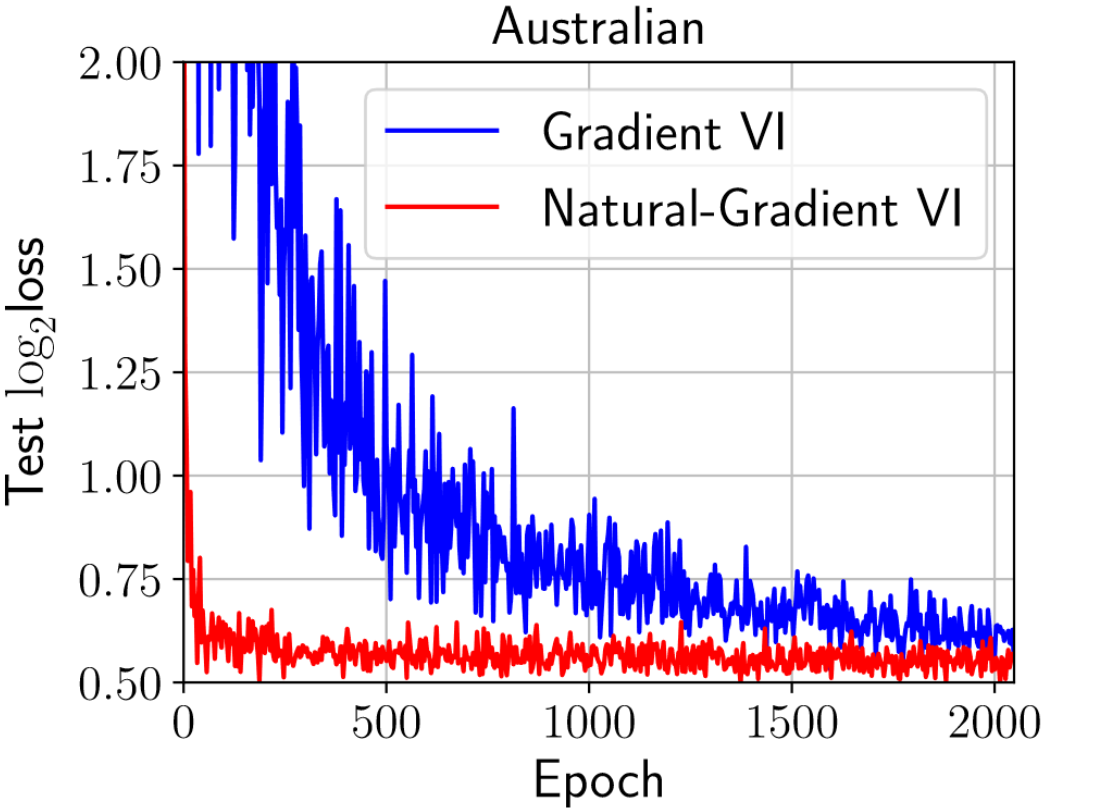
So how does this perform in practice? We explore this in detail in the second part of the blog. For now, we borrow Figure 1(b) from Khan & Nielsen (2018), which shows how Natural-Gradient VI (VOGN) can converge much quicker than Gradient VI (implemented as Bayes-By-Backprop (Blundell et al., 2015)) on two relatively small datasets.

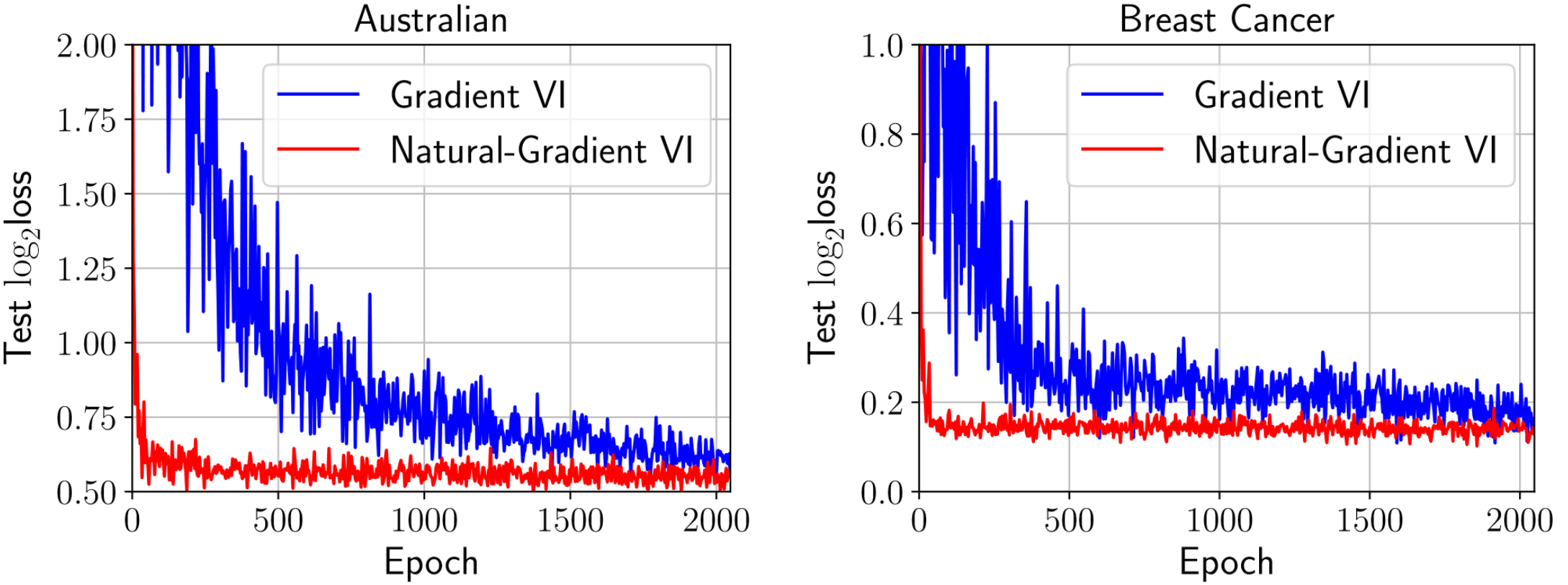
Figure 1: VOGN can converge quickly.

We’re done!

I hope you now understand NGVI for BNNs a little better. You have seen how the equations are derived, and hopefully have more of a feel for why and when they might work. There was a lot of detailed maths, but I have tried to provide some intuition and make all our approximations clear.

In this first part, we stopped at VOGN on small neural networks. In the second part, we will compare VOGN with stochastic gradient-based algorithms such as SGD and Adam to provide some further intuition. We will take some inspiration from Adam to scale VOGN to much larger datasets/architectures, such as ImageNet/ResNets. The next blog post will be a lot less mathematical!

If you would like to cite this blog post, you can use the following bibtex:

@misc{swaroop_2021, title={Natural-Gradient Variational Inference}, url={https://mlg-blog.com/2021/04/13/ngvi-bnns-part-1.html}, author={Swaroop, Siddharth}, year={2021}}