Image by Osawa et al. (2019).

Natural-Gradient Variational Inference 2: ImageNet-scale

Bayesian inference deep learning

In our previous post, we derived a natural-gradient variational inference (NGVI) algorithm for neural networks, detailing all our approximations and providing intuition. We saw it converge faster than more naive variational inference algorithms on relatively small-scale data. But a couple of key questions remain:

1. Can we scale such algorithms to very large datasets and architectures?
2. Did we gain anything from having additional Bayesian principles, or put differently, do we have better performance than SGD or Adam?

We tackle these questions in this second part of the natural-gradient for variational inference series. We show that we can get good performance at large scales with Bayesian principles, while maintaining reasonable uncertainties. We start by focussing on question (i): the issue of scalability. We notice similarities between our NGVI algorithm and Adam, and exploit this to borrow tricks that the community has developed for Adam over many years. This allows us to scale up to very large datasets/architectures. We then turn our focus to question (ii): have we improved on neural networks’ poorly-calibrated uncertainties thanks to our Bayesian thinking? We will see some benefits. Along the way, we will discuss the price we pay for them.

This second part of the blog closely follows a paper I was involved in, Practical Deep Learning with Bayesian Principles (Osawa et al., 2019). There is also a codebase if you are interested in experimenting with our algorithm, VOGN (Variational Online Gauss-Newton). As a postscript to this blog post, we summarise some good practices for training your own neural network with VOGN. $\newcommand{\vparam}{\boldsymbol{\theta}}$ $\newcommand{\veta}{\boldsymbol{\eta}}$ $\newcommand{\vphi}{\boldsymbol{\phi}}$ $\newcommand{\vmu}{\boldsymbol{\mu}}$ $\newcommand{\vSigma}{\boldsymbol{\Sigma}}$ $\newcommand{\vm}{\mathbf{m}}$ $\newcommand{\vF}{\mathbf{F}}$ $\newcommand{\vI}{\mathbf{I}}$ $\newcommand{\vg}{\mathbf{g}}$ $\newcommand{\vH}{\mathbf{H}}$ $\newcommand{\vs}{\mathbf{s}}$ $\newcommand{\myexpect}{\mathbb{E}}$ $\newcommand{\pipe}{\,|\,}$ $\newcommand{\data}{\mathcal{D}}$ $\newcommand{\loss}{\mathcal{L}}$ $\newcommand{\gauss}{\mathcal{N}}$

VOGN vs Adam

We start with the equations for the VOGN algorithm, derived in our previous blog post. This also serves as a quick summary of notation: please look at the previous blog post if anything is unclear! (Colours are purely for illustrative purposes.)

\begin{align} \label{eq:VOGN_mu} \vmu_{t+1} &= \vmu_t - \alpha_t \frac{ {\color{purple}\hat{\vg}(\vparam_t)} + {\color{blue}\tilde{\delta}}\vmu_t}{\vs_{t+1} + {\color{blue}\tilde{\delta}}}, \newline \label{eq:VOGN_Sigma} \vs_{t+1} &= (1-\beta_t)\vs_t + \beta_t \frac{1}{M} \sum_{i\in\mathcal{M}_t}\left( {\color{purple}\vg_i(\vparam_t)} \right)^2. \end{align}

Remember, we are updating the parameters of our (mean-field Gaussian) approximate posterior $q_t(\vparam)=\gauss(\vparam; \vmu_t, \vSigma_t)$, where $\vparam$ are the parameters of a neural network. We do this by iteratively updating two vectors, $\vmu_t$ and $\vs_t$, where $t$ indexes the iteration. We have a zero-mean prior $p(\vparam) = \gauss(\vparam; \color{blue}\boldsymbol{0}, {\color{blue}\delta^{-1}} \vI)$, and ${\color{blue}\tilde{\delta}} = {\color{blue}{\delta}} / N$. Our dataset consists of $N$ data examples, and we are taking per-example gradients of the negative log-likelihood $\color{purple}\vg_i(\vparam_t)$ at a sample from our current approximate posterior, $\vparam_t \sim q_t(\vparam)$. For a randomly-sampled minibatch $\mathcal{M}_t$ of size $M$, we have defined the average gradient ${\color{purple}\hat{\vg}(\vparam_t)} = \frac{1}{M}\sum_{i\in\mathcal{M}_t} {\color{purple}\vg_i(\vparam_t)}$. There is a simple relation between $\vSigma_t$ and $\vs_t$, $\vSigma_t^{-1} = N\vs_t + {\color{blue}\delta \vI}$. Finally, $\alpha_t>0$ and $0<\beta_t<1$ are learning rates, and all operations are element-wise.

It turns out that this update equation is very similar to Adam (Kingba & Ba, 2015). To see this, let’s write down the form that commonly-used optimisers take, such as SGD, RMSProp (Hinton, 2012), and Adam:

\begin{align} \label{eq:Adam_mu} \vmu_{t+1} &= \vmu_t - \alpha_t \frac{ {\color{purple}\hat{\vg}(\vmu_t)} + {\color{blue}\delta}\vmu_t} {\sqrt{\vs_{t+1}} + \epsilon}, \newline \label{eq:Adam_Sigma} \vs_{t+1} &= (1-\beta_t)\vs_t + \beta_t \left( \frac{1}{M} \sum_{i\in\mathcal{M}_t} {\color{purple}\vg_i(\vmu_t)} + {\color{blue}\delta} \vmu_t \right) ^2, \end{align}

where $\delta>0$ is our weight-decay regulariser, and $\epsilon>0$ is a small scalar constant. Immediately we can see striking similarities in the overall form of the equations! Let’s take a closer look at the similarities and differences:

1. Similarity: Both updates for $\vmu_t$ are similar, of the form $\vmu_{t+1} = \vmu_t - \alpha_t (\hat{\vg} + \delta \vmu_t) / \mathrm{function}{(\vs_{t+1})}$.
2. Difference: The denominator in the update for the means is slightly different. VOGN uses $(\vs_{t+1} + \tilde{\delta})$, while Adam has a square root, $\sqrt{\vs_{t+1}}$.
3. Difference: VOGN calculates gradients at a sample $\vparam_t \sim q_t(\vparam)$, while Adam calculates gradients just at the mean $\vmu_t$. In fact, when we remove this difference, we get a deterministic version of VOGN, which we call OGN.
4. Similarity: Both updates for $\vs_t$ take the form of a moving average update.
5. Difference: VOGN uses a Gauss-Newton approximation, requiring $\sum_i (\vg_i)^2$, while Adam (and other SGD-based algorithms) use a gradient-magnitude, $\left( \sum_i \vg_i \right) ^2$. Note that in VOGN, the sum is outside the square, while in SGD-based algorithms, the sum is inside the square.

The Gauss-Newton approximation (Difference 5) is a better approximation to second-order information (Hessian) than the gradient-magnitude approach. This better approximation is likely why VOGN does not require a square root over $\vs_{t+1}$ in the update for the means (Difference 2). However, calculating the Gauss-Newton approximation requires additional computation in frameworks such as PyTorch, leading to VOGN being slower (per epoch) compared to Adam. This is despite using speed-up tricks (Goodfellow, 2015).

The similarities in the equations indicate that we might be able to take techniques people use to scale Adam up to large datasets and architectures, and apply similar ideas to scale VOGN up. We can use batch normalisation, momentum, clever initialisations, data augmentation, learning rate scheduling, and so on.

Borrowing existing deep-learning techniques

Let’s go over a list of each of the changes we make, providing some intuition for them. Please see Osawa et al. (2019) for further details. Using all these techniques, we are able to scale VOGN to datasets like CIFAR-10 and ImageNet, and architectures such as ResNets.

1. Batch normalisation and momentum

Batch normalisation (Ioffe & Szegedy, 2015) empirically speeds up and stabilises training of neural networks. We can use BatchNorm layers as is normal in deep learning. In fact, in our VOGN implementation, we found that we do not have to maintain uncertainty over BatchNorm parameters.

We can also use momentum for VOGN in a similar way to Adam: we introduce momentum on $\vmu_t$, along with a momentum rate.

2. Initialisation

Over many years of training neural networks with SGD and Adam, the community has found tricks to speed up training using clever initialisation. We can get these same benefits by changing VOGN to look more like Adam at initialisation, before slowly relaxing our algorithm to become the full VOGN algorithm later in training.

This is achieved by introducing a tempering parameter $\tau$ in front of the KL term in the ELBO, which propagates its way through to the VOGN equations. To see exactly where $\tau$ crops up, please look at Equation 4 from Osawa et al. (2019), or see Algorithm 1 below. As $\tau\rightarrow 0$, we (loosely speaking) get more similar to Adam. So, at the beginning of training, we initialise $\tau$ at something small (like $0.1$) and increase to $1$ during the first few optimisation steps.

Other initialisations are the same as Adam: $\vmu_t$ is initialised using init.xavier_normal from PyTorch (Glorot & Bengio, 2010) and the momentum term is initialised to zero, like in Adam. VOGN’s $\vs_t$ is initialised using an additional forward pass through the first minibatch of data.

3. Learning rate scheduling

We can use learning rate scheduling for $\alpha_t$ exactly like is used for Adam and SGD at a large scale. We regularly decay the learning rate by a factor (typically a factor of 10).

4. Data augmentation

When training on image datasets, data augmentation (DA) can improve performance drastically. For example, we can use random cropping and/or random horizontal flipping of images.

Unfortunately, directly applying DA to VOGN does not lead to improvements, and also negatively affects uncertainty calibration. But we note that DA can be viewed as increasing the effective size of our dataset: remember that our dataset size $N$ affects VOGN (as opposed to Adam and SGD, where $N$ does not appear, as it unidentifiable with the weight-decay factor). So, we view DA as increasing $N$ by some factor depending on the exact DA technique: for example, if we horizontally flip each image with a probability of 50%, we increase $N$ by a factor of 2.

This is still a heuristic, and not mathematically rigorous. It seems to work quite well in our experiments, but requires further theoretical investigation. It is also closely related to KL-annealing in variational inference, as well as the recently-termed ‘cold posterior effect’ (Wenzel et al., 2020; Loo et al., 2021; Aitchison, 2021).

5. Distributed training

We would like to use multiple GPUs in parallel to perform large experiments quickly. Typically, we would just parallelise data, splitting up large minibatch sizes by sending different data to different GPUs. With VOGN, we can also parallelise computation over Monte-Carlo samples $\vparam_t \sim q_t(\vparam)$. Every GPU can use a different sample $\vparam_t$. This reduces variance during training, and we empirically find it leads to quicker convergence.

6. External damping factor

We introduce an external damping factor $\gamma$, added to $\vs_{t+1}$ in the denominator of Equation \eqref{eq:VOGN_mu} (Zhang et al., 2018). This increases the lower bound of the eigenvalues on the diagonal covariance $\vSigma_t$, preventing the step size and noise from becoming too large. However, this also detracts from the principled variational inference equations, and there is currently no theoretical justification for this (beyond the intuition we just provided).

Final algorithm

Let’s recap. We derived the VOGN equations (Equations \eqref{eq:VOGN_mu} and \eqref{eq:VOGN_Sigma}) in the previous blog post. We started this post by comparing the equations to Adam, noting key similarities and differences. One key difference was based off the Gauss-Newton approximation, which slows VOGN down (per epoch) compared to SGD-based algorithms like Adam. Based on the similarities, we borrowed tricks to scale Adam to large data settings, and applied them to VOGN.

All of these tricks are important to get VOGN’s results on ImageNet. The final algorithm is summarised in Algorithm 1 below. One downside of VOGN when compared to Adam is the additional hyperparameters that require tuning. At the end of this blog post, we provide best practices for tuning these hyperparameters.

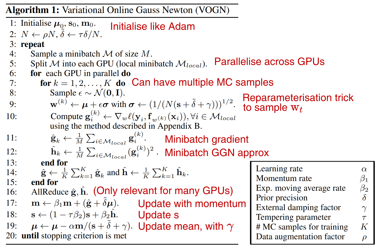
Algorithm 1: Final algorithm, ready for running on ImageNet. Additional notes explaining key steps are in red. The vanilla VOGN equations (Equations \eqref{eq:VOGN_mu} and \eqref{eq:VOGN_Sigma}) are in Steps 8–12 & 18–19. The final list of hyperparameters are summarised in the bottom right. The final four hyperparameters are specific to VOGN, and we provide best practices for tuning them at the end of the blog post.

Results on ImageNet

We are finally in a place to run VOGN on ImageNet and analyse results. We take Algorithm 1and run it on ImageNet.

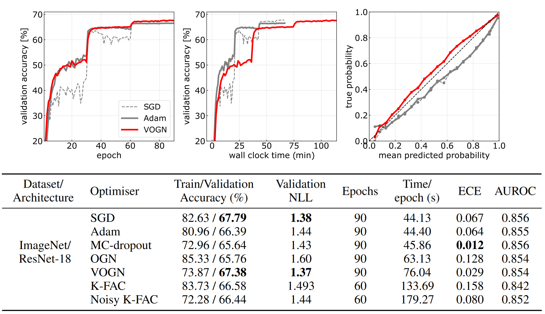
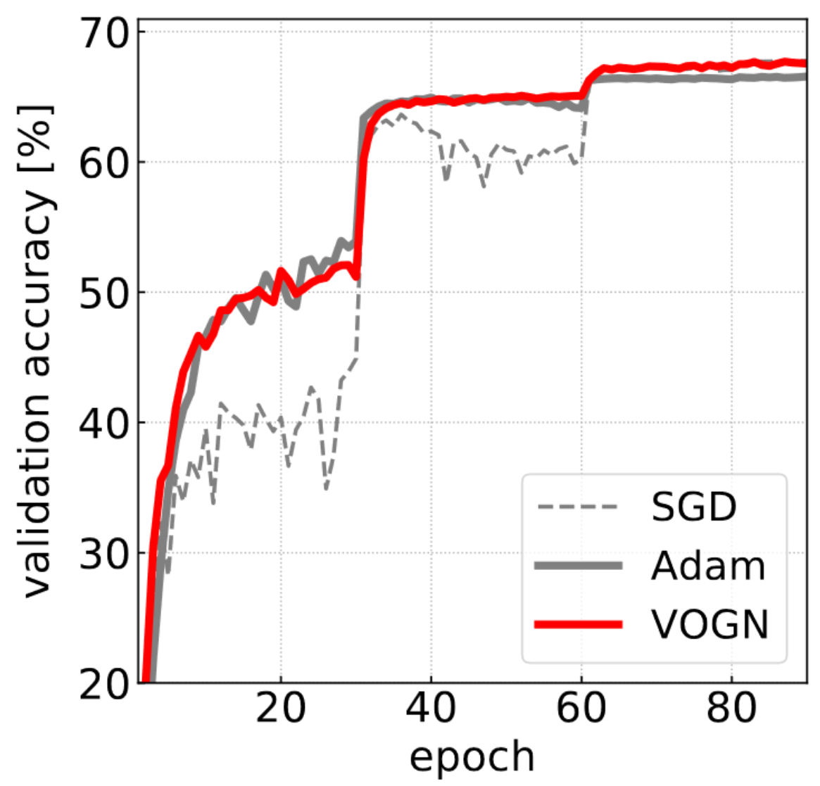
Figure 1: Results on ImageNet. VOGN converges in about as many epochs as Adam and SGD (top left plot), but is almost twice as slow per epoch (top middle plot). VOGN's calibration is better (top right plot). Overall, VOGN gets good accuracy and uncertainty metrics. See the paper for standard deviations over many runs.

Let’s go through these results slowly.

• Top left plot: VOGN’s convergence rate (per epoch) is very similar to Adam’s. The step increases (at epochs 30 and 60) are due to learning rate scheduling, which is best practice for training algorithms on ImageNet.
• Top middle plot: VOGN is about twice as slow (total time) compared to SGD and Adam. This is impressive compared to other approaches like Bayes-By-Backprop (Blundell et al., 2015), which currently can’t scale to ImageNet even if given an order of magnitude more time!
• Top right plot: In this calibration curve, the red line is closer to the diagonal than the other lines, showing better calibration. This plot is summarised in the ECE (Expected Calibration Error) column in the Table, where VOGN is better than SGD and Adam.
• Turning our attention to the Table, MC-dropout gets very good ECE, but this is at the cost of validation accuracy, and only achieved after a fine-grain sweep of hyperparameters (specifically the dropout rate, see Appendix G in the paper).
• OGN is a deterministic version of VOGN, where we do not use the reparameterisation trick to sample $\vparam_t$ during training (Steps 8 & 9 in Algorithm 1), and instead just use the mean $\vmu_t$.
• K-FAC has a Kronecker-factored structure as in Osawa et al. (2018), where they impressively trained on ImageNet in very few iterations. This blog post provides an introduction to K-FAC at a large scale.
• OGN and K-FAC perform well, but their metrics (particularly validation accuracy, validation negative-log-likelihood and ECE) are worse than VOGN.
• Noisy K-FAC (Zhang et al., 2018) takes a similar algorithm to VOGN and adds K-FAC structure to the covariance matrix. It is therefore more computationally expensive than VOGN (slower per epoch and total training time), but requires fewer epochs. It performs decently, but not as well as VOGN in this experiment.

There are many more results in Osawa et al. (2019), such as CIFAR-10 with a variety of architectures. We tend to see a similar story, where VOGN performs comparably on validation accuracy, and well on uncertainty metrics.

Some Bayesian trade-offs

Due to the Bayesian nature of VOGN, we see some interesting trade-offs (see the paper for figures).

1. Reducing the prior precision $\delta$ results in higher validation accuracy, but also a larger train-test gap, corresponding to more overfitting. With very small prior precisions, performance is similar to non-Bayesian methods like Adam.

2. Increasing the number of training MC samples ($K$ in Algorithm 1) improves VOGN’s convergence rate and stability, as it reduces gradient variance during training. But this is at the cost of increased computation. Increasing the number of MC samples during testing improves generalisation.

Downstream uncertainty performance

If you are like me, metrics such as negative-log-likelihood and expected calibration error do not mean much when it comes to analysing if your algorithm has ‘better uncertainty’. We should also test on downstream tasks to see how reliable our methods are, and more and more papers are starting to do so (see also this year’s NeurIPS Bayesian Deep Learning workshop, which makes this a priority). The VOGN paper tested on two downstream tasks: continual learning and out-of-distribution performance.

Continual Learning: I personally think continual learning is a very good way to test approximate Bayesian inference algorithms, particularly variational deep-learning algorithms. We tested VOGN on Permuted MNIST, finding it performs as well as VCL (Nguyen et al., 2018; Swaroop et al., 2019), but trained more than an order of magnitude quicker. More recently, VOGN has also achieved good results on a bigger Split CIFAR benchmark (see Section 4.5 of Eschenhagen (2019)), which VCL struggles to scale to.

Out-of-distribution performance: We also tested VOGN on standard out-of-distribution benchmarks, such as training on CIFAR-10 and testing on SVHN and LSUN. Figure 5 in the paper shows results (histograms of predictive entropy), where we qualitatively see VOGN performing well.

Conclusions and further reading

In the first blog post, we derived VOGN, our natural-gradient variational inference algorithm. In this blog post, we scaled it all the way to ImageNet. We made approximations along the way, but by being clever about when and where to make approximations, we have ended up with a practical algorithm that has Bayesian principles. Our final algorithm therefore performs reasonably well in downstream tasks.

It has been two years since publishing VOGN’s performance on ImageNet, and the field continues to move at break-neck pace. More algorithms and more benchmarks continue to be published, as well as more insight into VI.

• If you are interested in the maths of improving natural-gradient variational inference algorithms, I particularly recommend work by Wu Lin and co-authors. They looked at improving VON (same as VOGN but without the Gauss-Newton matrix approximation), deriving another quick NGVI algorithm that can perform well (Lin et al., 2020). They have also expanded to mixtures of exponential family distributions (Lin et al., 2019), and looked at structured natural gradient descent, drawing links to Newton-like algorithms (Lin et al., 2021).
• There is also interesting work looking at pathologies of mean-field VI on neural networks (VOGN is a mean-field VI algorithm). There are problems in the single-hidden-layer setting (Foong et al., 2020), and problems in the wide limit (Coker et al., 2021).

Acknowledgements

Firstly, many thanks to my co-authors Kazuki Osawa, Anirudh Jain, Runa Eschenhagen, Richard Turner, Rio Yokota and Emtiyaz Khan, many of whom also provided valuable feedback on these blog posts. I would also like to thank Andrew Foong, Wessel Bruinsma and Stratis Markou for their comments during drafting of these blog posts.

Post-scipt: A guide on how to tune VOGN

As we saw in Algorithm 1, there are many hyperparameters that need tuning for VOGN (and generally for VI at a large-scale). Here we briefly summarise how we did this in Osawa et al. (2019), following the guidelines presented in Section 3 of the paper. The key idea is to make sure VOGN training closely follows Adam’s trajectory in the beginning of training.

1. First, we tune hyperparameters for OGN, which is the same as VOGN except setting $\vparam_t=\vmu_t$ (no MC sampling). OGN is more stable than VOGN and is a convenient stepping stone as we move from Adam to VOGN. So, we initialise OGN’s hyperparameters at Adam’s values, and tune until OGN is competitive with Adam. This requires tuning learning rates, prior precision $\delta$, and setting a suitable value for the data augmentation factor (if using data augmentation).

2. Then, we move to VOGN. Now, we (fine-)tune the prior precision $\delta$, warm-start the tempering parameter $\tau$ (such as increasing $\tau$ from $0.1\rightarrow1$ during the first few optimisation steps), and the number of MC samples $K$ for VOGN (more samples means more stable training, but more computation cost). We also now consider adding an external damping factor $\gamma$ if required.