Bayesian Deep Learning via Subnetwork Inference

Bayesian inference deep learning

Motivation: Bayesian deep learning is important but hard

Despite their successes, accurately quantifying uncertainty in the predictions of DNNs is notoriously hard, especially if there is a shift in the data distribution between train and test time. In practice, this might often lead to overconfident predictions, which is particularly harmful in safety-critical applications such as healthcare and autonomous driving. One principled approach to quantify the predictive uncertainty of a neural net is to use Bayesian inference.

The standard practice in deep learning is to estimate the parameters using just a single point found through gradient-based optimisation. In contrast, in Bayesian deep learning (check out this blog post for an introduction to Bayesian deep learning), the goal is to infer a full posterior distribution over the model’s weights. By capturing a distribution over weights, we capture a distribution over neural networks, which means that prediction essentially takes into account the predictions of (infinitely) many neural networks. Intuitively, on data points that are very distinct from the training data, these different neural nets will disagree on their predictions. This will result in high predictive uncertainty on such data points and therefore reduce overconfidence.

The problem is that modern deep neural nets are so big that even trying to approximate this posterior is highly non-trivial. We are not even talking about humongous 100-billion-parameter models like OpenAI’s GPT-3 here (Brown et al., 2020) — even for a neural net with more than just a few layers it’s hard to do good posterior inference! Therefore, it’s becoming more and more challenging to design approximate inference methods that actually scale.

To cope with this problem, many existing Bayesian deep learning methods make very strong and unrealistic approximations to the structure of the posterior. For example, the common mean field approximation approximates the posterior by a distribution which fully factorises over individual weights. Unfortunately, recent papers (Ovadia et al., 2019; Foong et al., 2019) have empirically demonstrated that such strong assumptions result in bad performance on downstream tasks such as uncertainty estimation. Can we do better than this? $\newcommand{\vy}{\mathbf{y}}$ $\newcommand{\vw}{\mathbf{w}}$ $\newcommand{\mH}{\mathbf{H}}$ $\newcommand{\mX}{\mathbf{X}}$ $\newcommand{\D}{\mathcal{D}}$ $\newcommand{\c}{\textsf{c}}$

Idea: Do inference over only a small subset of the model parameters!

Most existing Bayesian deep learning methods try to do inference over all the weights of the neural net. But do we actually need to estimate a posterior distribution over all weights?

It turns out that you often don’t need all those weights. In particular, recent research (Cheng et al., 2017) has shown that, since deep neural nets are so heavily overparametrised, it’s possible to find a small subnetwork within a neural net containing only a very small fraction of the weights, which, miraculously, can achieve the same accuracy as the full neural net. These subnetworks can be found by so-called pruning techniques.

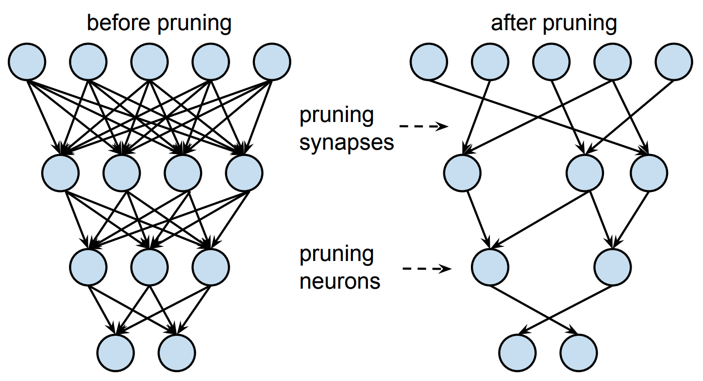
Figure 1: An illustration of neural network pruning (Han et al., 2015).

As shown in Figure 1, pruning techniques typically first train the neural net, and then, after training, remove certain weights or even entire neurons according to some criterion. There has been a lot of recent interest in this research direction; for example, the best paper award at ICLR 2019 went to Jonathan Frankle and Michael Carbin’s now famous work on the lottery ticket hypothesis (Frankle and Carbin, 2018), which showed that you can even retrain the pruned network from scratch and still achieve the same accuracy as the full network.

But how does this help us? We asked ourselves the exact same question about the model uncertainty: Can a full deep neural net’s model uncertainty be well-preserved by a small subnetwork’s model uncertainty? It turns out that the answer is yes, and in the remainder of this blog post, you will learn about how we came to this conclusion.

Our proposed approximation to the posterior

Assume that we have divided the weights $\vw$ into two disjoint subsets: (1) the subnetwork $\vw_S$ and (2) the set of all remaining weights $\{\vw_r\}_{r \in S^\c}$. We will later describe how we select the subnetwork; for now, just assume that we have it already. We propose to approximate the posterior distribution over as follows: \begin{equation} p(\vw \cond \D) \overset{\text{(i)}}{\approx} p(\vw_S \cond \D) \prod_{r \in S^\c} \delta(\vw_r - \widehat{\vw}_r) \overset{\text{(ii)}}{\approx} q(\vw_S) \prod_{r \in S^\c} \delta(\vw_r - \widehat{\vw}_r) =: q_S(\vw). \end{equation} The first step (i) of our posterior approximation then involves a posterior distribution over just the subnetwork $\vw_S$, and delta functions over all remaining weights $\{\vw_r\}_{r \in S^\c}$. Put differently, we only treat the subnetwork $\vw_S$ in a probabilistic way, and assume that each remaining weight $\vw_r$ is deterministic and set to some fixed value $\widehat\vw_r$. Unfortunately, exact inference over the subnetwork is still intractable, so, in the second step (ii) of our approximation, we introduce an approximate posterior $q$ over the subnetwork $\vw_S$. Importantly, as the subnetwork is much smaller than the full network, this allows us to use expressive posterior approximations that would otherwise be computationally intractable (e.g. full-covariance Gaussians). That’s it.

There are a few questions that we still need to answer:

1. How do we choose and infer the subnetwork posterior $q(\vw_S)$? That is, what form does $q$ have, and how do we infer its parameters?
2. How do we set the fixed values $\widehat\vw_r$ of all remaining weights $\{\vw_r\}_{r \in S^\c}$?
3. How do we select the subnetwork $\vw_S$ in the first place?
4. How do we make predictions with this approximate posterior?
5. How does subnetwork inference perform in practice?

Let’s start with Q1.

Q1. How do we choose and infer the subnetwork posterior ?

In this work, we infer a full-covariance Gaussian posterior over the subnetwork using the Laplace approximation, which is a classic approximate inference technique. If you don’t recall how the Laplace approximation works, below we provide a short summary. For more details on the Laplace approximation and a review of its use in deep learning, please refer to Daxberger et al. (2021).

The Laplace approximation proceeds in two steps.

1. Obtain a point estimate over all model weights using maximum a-posteriori (short MAP) inference. In deep learning, this is typically done using stochastic gradient-based optimisation methods such as SGD. \begin{equation} \widehat\vw = \argmax_{\vw} \, [\log p(\vy \cond \mX, \vw) + \log p(\vw)] \end{equation}

2. Locally approximate the log-density of the posterior with a second-order Taylor expansion. This produces a full-covariance Gaussian posterior over the weights, where the mean of the Gaussian is simply the MAP estimate, and the covariance matrix of the Gaussian is the inverse Hessian $\mH$ of the loss with respect to the weights $\vw$ (averaged over the training data points): \begin{equation} p(\vw \cond \D) \approx q(\vw) = \Normal(\vw \cond \widehat\vw, \mH^{-1}). \end{equation}

What this essentially does is it defines a Gaussian centered at the MAP estimate, with a covariance matrix that matches the curvature of the loss at the MAP estimate, as illustrated in Figure 2.

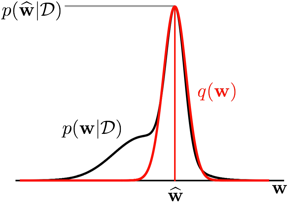
Figure 2: A conceptual illustration of the Laplace approximation in one dimension (image adapted with kind permission from Richard Turner). We plot the parameter $\mathbf{w}$ ($x$-axis) against the density of the true posterior $p(\mathbf{w}\cond\mathcal{D})$ (in black) as well as that of the corresponding Laplace approximation $q(\mathbf{w})$ (in red). As we can see, $q(\mathbf{w})$ is a Gaussian centered at the mode $\widehat{\mathbf{w}}$ of the posterior $p(\mathbf{w}\cond\mathcal{D})$, with covariance matrix matching the curvature of $p(\mathbf{w}\cond\mathcal{D})$ at $\widehat{\mathbf{w}}$.

The main advantage of the Laplace approximation, and also the reason why we use it, is that it is applied post-hoc on top of a MAP estimate and doesn’t require us to re-train the network. This is practically very appealing as MAP estimation is something we can do very well in deep neural nets. The main issue, however, is that it requires us to compute, store, and invert the full Hessian $\mH$ over all weights. This scales quadratically in space and cubically in time (in terms of the number of weights) and is therefore computationally intractable for modern neural nets.

Fortunately, in our case, we don’t actually want to do inference over all the weights, but only over a subnetwork. In this case, the second step of the Laplace approximation involves inferring a full-covariance Gaussian posterior over only the subnetwork weights $\vw_S$: \begin{equation} p(\vw_S \cond \D) \approx q(\vw_S) = \Normal(\vw_S \cond \widehat\vw_S, \mH_S^{-1}). \end{equation} This is now tractable, since the subnetwork will in practice be substantially smaller than the full network, effectively giving us quadratic gains in space complexity and cubic gains in time complexity!

Q2. How do we set the fixed values $\widehat{\mathbf{w}}_r$ of all remaining weights $\{\mathbf{w}_r\}_{r \in S^\c}$?

In fact, this also answers Q2 of how to set the remaining weights not part of the subnetwork: Since the Laplace approximation requires us to first obtain a MAP estimate over all weights, it’s natural to simply leave all other weights at their MAP estimates!

Let’s now look at how subnetwork inference is done in practice.

The full subnetwork inference algorithm

Overall, our proposed subnetwork inference algorithm comprises the following four steps:

1. Obtain a MAP estimate over all the weights of the neural net using standard optimisation methods such as SGD (see Figure 3).

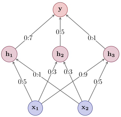
Figure 3: Step 1: Point estimation.

2. Select a small subnetwork (see Figure 4) — we’ll discuss in a second how this can be done in practice.

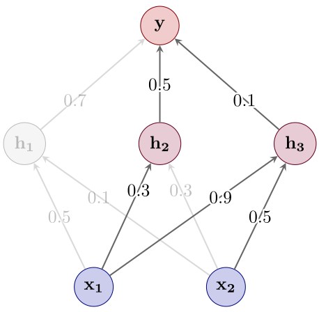
Figure 4: Step 2: Subnetwork selection.

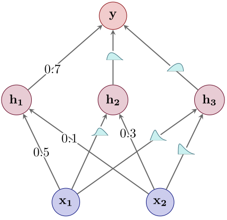
3. Perform Bayesian inference just over the subnetwork (see Figure 5). As described above, we use the Laplace approximation to infer a full-covariance Gaussian over the subnetwork, and leave all other weights at their MAP estimates.

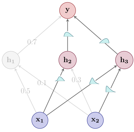
Figure 5: Step 3: Bayesian inference.

4. Lastly, use the resulting mixed probabilistic–deterministic model to make predictions (see Figure 6).

Figure 6: Step 4: Prediction.

Ok, now we know how to do inference over the subnetwork, but how do we find the subnetwork in the first place?

Q3. How do we select the subnetwork $\mathbf{w}_S$ in the first place?

Recall that we want to preserve as much model uncertainty as possible with our subnetwork. A natural goal is therefore to find the subnetwork whose posterior is closest to the full network posterior. That is, we want to find the subset of weights that minimises some measure of discrepancy between the posterior over the full network and the posterior over the subnetwork.

To measure this discrepancy, we choose to use the Wasserstein distance: \begin{align} &\min \text{Wass}[\ \text{exact full posterior}\ |\ \text{subnetwork posterior}\ ] \nonumber \vphantom{\prod} \newline &\qquad= \min \text{Wass}[\ p(\mathbf{w} \cond \mathcal{D})\ |\ q_S(\mathbf{w})\ ] \vphantom{\prod} \newline &\qquad\approx \min \text{Wass}[\ \mathcal{N}\left(\mathbf{w}; \widehat{\mathbf{w}}, \mathbf{H}^{-1}\right)\ |\ \mathcal{N}(\mathbf{w}_S; \widehat{\mathbf{w}}_S, \mathbf{H}_S^{-1}) \prod_{r \in S^\c} \delta(\mathbf{w}_r - \widehat{\mathbf{w}}_r )\ ]. \end{align} As the exact full network posterior $p(\mathbf{w} \cond \mathcal{D})$ is intractable, we here approximate it as a Gaussian $\mathcal{N}\left(\mathbf{w}; \widehat{\mathbf{w}}, \mathbf{H}^{-1}\right)$ over all weights (also estimated via the Laplace approximation). Also, as described earlier, the subnetwork posterior $q_S(\mathbf{w})$ is composed of a Gaussian $\mathcal{N}(\mathbf{w}_S; \widehat{\mathbf{w}}_S, \mathbf{H}_S^{-1})$ over the subnetwork and delta functions $\delta(\mathbf{w}_r - \widehat{\mathbf{w}}_r )$ over all other weights $\{\mathbf{w}_r\}_{r \in S^\c}$. Note that due to the delta functions, the subnetwork posterior is degenerate; this is why we use the Wasserstein distance, which remains well-defined for such degenerate distributions.

Unfortunately, this objective is still intractable, as it depends on all entries of the Hessian of the full network. To obtain a tractable objective, we assume that the full network posterior is factorised. By making this factorisation assumption, the Wasserstein objective now only depends on the diagonal entries of the Hessian, which are cheap to compute. I know what you’re thinking right now: “Didn’t they just tell us that the whole point of this subnetwork inference thing is to avoid making the assumption that the posterior is diagonal? And now they’re telling us that, actually, we still do have to make this assumption? This doesn’t make any sense!”

Well, in fact, it turns out that making the diagonal assumption just for the purpose of subnetwork selection, but then doing full-covariance Gaussian posterior inference over the subnetwork is much better than making the diagonal assumption for the purpose of inference itself (i.e. inference over the weights of the subnetwork and even over all weights), which we’ll see in the experiments later.

All in all, our proposed subnetwork selection procedure is as follows:

1. Estimate a factorised Gaussian posterior over all weights, using for example a diagonal Laplace approximation.
2. Select those weights with the largest marginal variances. Why the weights with largest marginal variances? Well, one can show that, under the diagonal assumption, those are the weights that minimise the Wasserstein objective defined above.

Q4. How do we make predictions with this approximate posterior?

Great, we now know that a subnetwork can be found by (approximately) minimising the Wasserstein distance between the subnetwork posterior and the full network posterior. But how do we make predictions with this weird approximate posterior that is partly probabilistic and partly deterministic? We simply use all the weights of the neural net to make predictions: we integrate out the weights in the subnetwork, and just leave all other weights fixed at their MAP estimates. For integrating out the subnetwork weights, one can either use Monte Carlo or a closed-form approximation — please refer to the full paper for more details (the reference is given at the end of this blog post). Subnetwork inference therefore combines the strong predictive accuracy of the MAP estimate with the calibrated uncertainties of a Bayesian posterior.

Finally, we will now demonstrate the effectiveness of subnetwork inference in two experiments.

Q5. How does subnetwork inference perform in practice?

Experiment 1: How does subnetwork inference preserve predictive uncertainty?

In the first experiment we train a small, 2-layer, fully-connected network with a total of 2600 weights on a 1D regression task, shown in Figure 7.

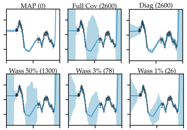
Figure 7: Predictive distributions (mean $\pm$ std) for 1D regression. The numbers in parentheses denote the number of parameters over which inference was done (out of 2600 in total). Wasserstein subnetwork inference maintains richer predictive uncertainties at smaller parameter counts.

The number in brackets in the plot title denotes the number of weights over which we do inference; for example, for the MAP estimate (Figure 7, top left), inference was done over zero weights. As you can see, the 1D function we’re trying to fit consists of two separated clusters of data, and the goal here is to capture as much of the predictive uncertainty as possible, especially in-between those data clusters (Foong et al., 2019). As expected, the point estimate (Figure 7, top left) doesn’t capture any uncertainty, but instead makes confident predictions even in regions where there’s no data, which is bad.

On the other extreme, we can infer a full covariance Gaussian posterior over all the 2600 weights using a Laplace approximation (Figure 7, top middle), which is only tractable here due to the small model size. As we can see, a full-covariance Gaussian posterior is able to capture predictive uncertainty both at the boundaries and in-between the data clusters, so we will consider this to be the ideal, ground-truth posterior for this experiment.

Of course, in larger-scale settings, a full-covariance Gaussian would be intractable, so people often resort to diagonal approximations which assume full independence between the weights (Figure 7, top right). Unfortunately, as we can see, even though we do inference over all 2600 weights, due to the diagonal assumption we sacrifice a lot of the predictive uncertainty, especially in-between the two data clusters, where it’s only marginally better than the point estimate.

Now what about our proposed subnetwork inference method? First, let’s try doing full-covariance Gaussian inference over only 50% (that is, 1300) of the weights, found using the described Wasserstein minimisation approach (Figure 7, bottom left). As we can see, this approach captures predictive uncertainty much better than the diagonal posterior, and is even quite close to the full-covariance Gaussian over all weights. Well, but 50% is still quite a lot of weights, so let’s try to go even smaller, much smaller, to only 3% of the weights, which corresponds to just 78 weights here (Figure 7, bottom middle). Even then, we’re still much better off than the diagonal Gaussian. Let’s push this to the extreme, and estimate a full-covariance Gaussian over as little as 1% (that is, 26) of the weights (Figure 7, bottom right). Perhaps surprisingly, even with 1% of weights remaining, we do significantly better than the diagonal baseline, and are able to capture significant in-between uncertainty!

Overall, the take-away from this experiment is that doing expressive inference over a very small, but carefully chosen subnetwork, and capturing weight correlations just within that subnetwork can preserve more predictive uncertainty than a method that does inference over all the weights, but ignores weight correlations.

Experiment 2: How robust is subnetwork inference to distribution shift?

Ok, 1D regression is fun, but we’re of course interested in scaling this to more realistic settings. In this second experiment, we consider the task of image classification under distribution shift. This task is much more challenging than 1D regression, so the model that we use is significantly larger than before: we use a ResNet-18 model with over 11 million weights, and, to remain tractable, we do inference over as little as 42 thousand (which is only around 0.38%) of the weights, again found using Wasserstein minimisation.

We consider five baselines: the MAP estimate, a diagonal Laplace approximation over all 11M weights, Monte Carlo (MC) dropout over all weights (Gal and Ghahramani, 2015), Variational Online Gauss-Newton (short VOGN, Osawa et al., 2019), which estimates a factorised Gaussian over all weights, a Deep Ensemble (Lakshminarayanan et al., 2017) of 5 independently trained ResNet-18 models, and Stochastic Weight Averaging Gaussian (short SWAG, Maddox et al., 2019), which estimates a low-rank plus diagonal posterior over all weights. As another baseline, we also consider subnetwork inference with a randomly selected subnetwork (denoted Ours (Rand)), which will allow us to assess the impact of how the subnetwork is chosen.

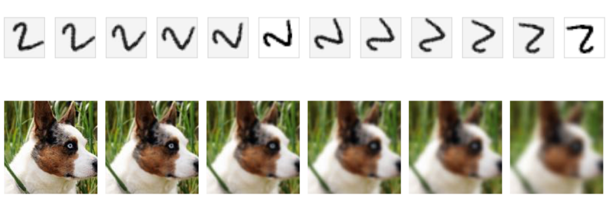
Figure 8: Example images from the (top) rotated MNIST and (bottom) corrupted CIFAR-10 benchmarks. (Top) An image of the digit 2 is increasingly rotated. (Bottom) An image of a dog is increasingly blurred.

We consider two benchmarks for evaluating robustness to distribution shift which were recently proposed by Ovadia et al. (2019) (Figure 8): firstly, we have rotated MNIST, where the model is trained on the standard MNIST training set, and then at test time evaluated on increasingly rotated MNIST digits (as for example shown for the digit 2 in Figure 8, top); and secondly, we consider corrupted CIFAR-10, where we again train on the standard CIFAR-10 training set, but then evaluate on corrupted CIFAR-10 images; the test set contains over a dozen different corruption types, with five levels of increasing corruption severity (in this example, the image of a dog in Figure 8, bottom, is getting more and more blurry from left to right).

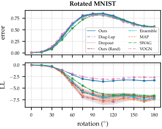
Figure 9: Results on the rotated MNIST benchmark, showing the mean $\pm$ std of the test error (top) and log-likelihood (bottom) across three different seeds. Subnetwork inference achieves better uncertainty calibration and robustness to distribution shift than point-estimated networks and other Bayesian deep learning approaches (except for VOGN), while retaining accuracy.

Let’s start with rotated MNIST (Figure 9). On the x-axis, we have the degree of rotation, and on the y-axis, we plot two different metrics: on top, we plot the test errors achieved by the different methods (where lower values are better), and on the bottom, we plot the corresponding log-likelihood, as a measure of calibration (where higher values are better). Here, we see that MAP, diagonal Laplace, MC dropout, the deep ensemble, SWAG, and the random subnetwork baseline all perform roughly similarly in terms of calibration (Figure 9, bottom): their calibration becomes worse as we increase the degree of rotation; in contrast to that, subnetwork inference (shown in dark blue) remains much better calibrated, even at high degrees of rotation. The only competitive method here is VOGN, which slightly outperforms subnetwork inference in terms of calibration. Importantly, observe that this increase in robustness does not come at cost of accuracy (Figure 9, top): Wasserstein subnetwork inference (as well as VOGN) retain the same accuracy as the other methods.

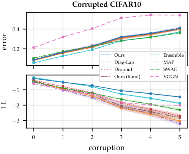
Figure 10: Results on the corrupted CIFAR-10 benchmark, showing the mean $\pm$ std of the test error (top) and log-likelihood (bottom) across three different seeds. Subnetwork inference achieves better uncertainty calibration and robustness to distribution shift than point-estimated networks and other Bayesian deep learning approaches, while retaining accuracy.

Now let’s look at corrupted CIFAR10 (Figure 10). There, the story is somewhat similar: we plot the corruption severity on the x-axis versus the error (Figure 10, top) and log-likelihood (Figure 10, bottom) on the y-axis. Here, MAP, diagonal Laplace, MC dropout and the random subnetwork baseline are all poorly calibrated (Figure 10, bottom). VOGN, SWAG and deep ensembles are a bit better calibrated, but are still significantly outperformed by subnetwork inference (again in dark blue), even at high corruption severities. Importantly, the improved robustness of Wasserstein subnetwork inference again does not compromise accuracy (Figure 10, top). In contrast, the accuracy of VOGN suffers on this dataset.

Overall, the take-away from this experiment is that subnetwork inference is better calibrated and therefore more robust to distribution shift than state-of-the-art baselines for uncertainty estimation in deep neural nets.

Take-home message

To conclude, in this blog post, we described subnetwork inference, which is a Bayesian deep learning method that does expressive inference over a carefully chosen subnetwork within a neural network. We also showed some empirical results suggesting that this works better than doing crude inference over the full network. There remain clear limitations of this work that deserve more investigation in the future: The most important one is to develop better subnetwork selection strategies that avoid the potentially restrictive approximations we use (i.e. the diagonal approximation to the posterior covariance matrix).

Thanks a lot for reading this blog post! If you want to learn more about this work, please feel free to check out our full ICML 2021 paper:

• Erik Daxberger, Eric Nalisnick, James Urquhart Allingham, Javier Antorán, José Miguel Hernández-Lobato. Bayesian Deep Learning via Subnetwork Inference. In ICML 2021.

Finally, we would like to thank Stratis Markou, Wessel Bruinsma and Richard Turner for many helpful comments on this blog post!